Diffusion, in general, is a concept which describes the propagation of particles over time within some substance. One good example is temperature diffusing in a closed body leading to the heat equation. The question hereby is: how does the temperature change over time at the considered spatial locations. Assuming for simplicity only 1D spatial locations, this can mathematically be described by a partial differential equation (PDE)
\begin{equation} \frac{\partial u(x,t)}{\partial t} = g \cdot \frac{\partial^2 u(x,t)}{\partial^2 x^2}. \label{eq:FEDIntroduction_PDE} \end{equation}with \(g\) being a constant describing the conductivity of the homogeneous diffusion (e.g. how fast levels the temperature to equality). I am not going into details here why this equation looks like it looks (check the linked video for a great introduction). My concern is more about the discretization of this PDE. By using the Euler method, the discretization is achieved by
\begin{align*} t_{k+1} &= t_k + \tau \\ \fvec{u}_{k+1} &= \fvec{u}_k + \tau \cdot (g \cdot \Delta \fvec{u}_k) \\ \end{align*}which proceeds over time in steps of \(\tau\). The part in the brackets is basically the discrete version of \eqref{eq:FEDIntroduction_PDE} where \(\Delta\) denotes an operator for the central finite difference approximation of the second order derivative \(\frac{\partial^2 u(x,t)}{\partial^2 x^2}\) applied to the vector of signal values \(\fvec{u}_k\)1 at the time \(t_k\) and the constant \(g\) is re-used as is. Note that in this explicit scheme the time step \(\tau\) is fixed over the complete process. But one step size might not be appropriate for every step; it may be better if some are larger and others are smaller. This problem is addressed by the Fast Explicit Diffusion (FED) algorithm. Basically, it introduces varying time steps \(\tau_i\) resulting in more accuracy and higher performance (hence the “Fast” in the name). This article has the aim to introduce FED and to provide examples of how it can be used.
Before going into the details, let me note that FED can not only be applied to homogeneous diffusions (like the heat equation) but also to inhomogeneous, anisotropic or isotropic and even multi-dimensional diffusion problems. More precisely, FED can be applied to any finite scheme of the form [12-13]2
\begin{equation} \fvec{u}_{k+1} = \left( I + \tau \cdot A \right) \cdot \fvec{u}_k \label{eq:FEDIntroduction_Arbitrary} \end{equation}where \(A\) is some symmetric and negative semidefinite matrix embedding the conductivity information. This includes the approximation of the second order derivative \(\Delta\) and the constant \(g\). I am coming to this point later, but first dive into what FED actually does.
The rest of this article is structured as follows: first, the concept behind FED is introduced by an example showing the basic rationale behind it. Next, the notation is simplified allowing for generalization of the concept behind FED to a wider range of problems. Then, a summary of the used parameters is given, and in the last section, some elaboration of the role of box filters in FED is provided.
How does it work?
For simplicity, I stick to one-dimensional homogeneous diffusion problems and set the constant to \(g = 1\). First, two important notes
- If a homogeneous diffusion is applied to a signal, it is equivalent to applying a Gaussian to that signal. More precisely, the total diffusion time \(T\) maps to a Gaussian with standard deviation \(\sigma = \sqrt{2 \cdot T}\) (e.g. Digital Image Processing by Burger and Burge, p. 435).
- If a filter whose coefficients are non-negative and sum up to 1 (i.e. \(\sum w_i = 1\)) is applied multiple times to a signal, it approximates a Gaussian convolution with that signal. This is known from the central limit theorem (CLT).
What has FED now to do with this? In essence, FED introduces an alternative way of applying such a filter by using iterations of explicit diffusion steps. The main finding is that filters (with the discussed properties) can be defined as
\begin{equation} B_{2n+1} = \prod_{i=0}^{n-1} \left( I + \tau_i \Delta \right). \label{eq:FEDIntroduction_Cycle} \end{equation}I directly try to be a bit more concrete here: \(B_{2n+1}\) denotes a box filter of size \(2n+1\) and \(I\) the identity (e.g. 1). \(\Delta\) is, again, the operator for an approximation of the second order derivative. If applied to a signal \(\fvec{u}\), it may be defined as3
\begin{equation} \Delta \fvec{u} = u(x-1, t) - 2 \cdot u(x, t) + u(x+1, t), \label{eq:FEDIntroduction_Delta} \end{equation}so the spatial difference at some fixed time \(t\). You can also think of this operation as a kernel \(\left( 1, -2, 1 \right)\) convolved with the signal \(\fvec{u}\). All iterations of \eqref{eq:FEDIntroduction_Cycle} together are called a FED cycle. Given this, there is only \(\tau_i\) left. This is actually the heart of FED since it denotes the varying step sizes, and in this case, is defined as
\begin{equation} \tau_i = \tau_{\text{max}} \cdot \frac{1}{2 \cos ^2\left(\frac{\pi (2 i+1)}{4 n+2}\right)} \label{eq:FEDIntroduction_TimeStepsBox} \end{equation}with \(\tau_{\text{max}} = \frac{1}{2}\) here (more on this parameter later). Unfortunately, I can't tell you why this works (the authors provide proves though [46 ff. (Appendix)]) but I can give an example.
We want to show that the FED cycle applied to the signal is indeed the same as convolving the signal with a box filter. Let's start by defining a small signal and a box filter of size \(n=1\)
\begin{equation*} \fvec{u} = \begin{pmatrix} 1 \\ 4 \\ 2 \\ 6 \\ \end{pmatrix} \quad \text{and} \quad \tilde{B}_3 = \frac{1}{3} \cdot \begin{pmatrix} 1 \\ 1 \\ 1 \\ \end{pmatrix}. \end{equation*}The convolution with reflected boundaries4 results in
\begin{equation} \fvec{u} * \tilde{B}_3 = \left( 2.,2.33333,4.,4.66667 \right)^T. \label{eq:FEDIntroduction_ExampleConvolution} \end{equation}For the FED approach, we first need to calculate the time step (only one in this case because of \(n=1\))
\begin{equation*} \tau_0 = \frac{1}{2} \cdot \frac{1}{2 \cos ^2\left(\frac{\pi (2 \cdot 0+1)}{4 1+2}\right)} = \frac{1}{3} \end{equation*}and then \eqref{eq:FEDIntroduction_Cycle} can be applied to \(u\) by multiplication resulting in the following explicit diffusion step
\begin{equation*} B_3 \cdot \fvec{u} = \prod_{i=0}^{1-1} \left( I + \tau_i \Delta \right) \cdot \fvec{u} = \fvec{u} + \tau_0 \cdot \Delta \fvec{u}. \end{equation*}How is \(\Delta \fvec{u}\) defined here? It is basically \eqref{eq:FEDIntroduction_Delta} but extended to handle out of border accesses correctly
\begin{equation*} \Delta u_{j} = \begin{cases} &-& u_{j} &+& u_{j+1}, & j=1 \\ u_{j-1} &-& u_{j}, & & & j=N \\ u_{j-1} &-& 2 u_{j} &+& u_{j+1}, & \text{else} \\ \end{cases} \end{equation*}and is applied to every vector component \(u_{j}\). In this case, we have
\begin{equation*} \Delta \fvec{u} = \begin{pmatrix} -1+4 \\ 1-2\cdot 4+2 \\ 4-2\cdot 2 + 6 \\ 2-6 \\ \end{pmatrix} = \begin{pmatrix} 3 \\ -5 \\ 6 \\ -4 \\ \end{pmatrix} \end{equation*}and then everything can be combined together
\begin{equation} \fvec{u} + \tau_0 \cdot \Delta \fvec{u} = \begin{pmatrix} 1 \\ 4 \\ 2 \\ 6 \\ \end{pmatrix} + \frac{1}{3} \cdot \begin{pmatrix} 3 \\ -5 \\ 6 \\ -4 \\ \end{pmatrix} = \begin{pmatrix} 2 \\ 2.33333 \\ 4 \\ 4.66667 \\ \end{pmatrix}. \label{eq:FEDIntroduction_ExampleFED} \end{equation}As you can see, \eqref{eq:FEDIntroduction_ExampleConvolution} and \eqref{eq:FEDIntroduction_ExampleFED} produce indeed identical results.
If larger filters and hence more iterations per FED cycle are needed, the same technique would be recursively applied. E.g. for \(n=2\) we get
\begin{equation*} B_5 \cdot \fvec{u}= \prod_{i=0}^{2-1} \left( I + \tau_i \Delta \right) \cdot \fvec{u} = \fvec{u} + \tau_0 \cdot \Delta \fvec{u} + \tau_1 \cdot \Delta \fvec{u} + \tau_0 \cdot \tau_1 \cdot \Delta (\Delta \fvec{u}), \end{equation*}where \(\Delta (\Delta \fvec{u})\) effectively encodes an approximation for the fourth order derivative (it calculates the second order derivative of something which is already the second order derivative of the input signal). The concept stays the same for larger filters. The iterations of the FED cycle gradually reach the same state of the corresponding box filter response. To visualize this, the following animation shows the result of a filter with \(n=10\) each time plotting the state up to the current iteration (i.e. the previous and current multiplications).
So far we only discussed exactly one FED cycle (which consists of iterations). It is also possible to apply multiple cycles just by repeating the procedure. This is then equal to iteratively applying multiple filters to the signal.
Recapitulate what we now have:
- multiple iterations (products in \eqref{eq:FEDIntroduction_Cycle}) form a FED cycle,
- a FED cycle is the same like convolving the signal with a (box) filter,
- multiple FED cycles are the same as the iterative convolution of the signal with (box) filters,
- applying multiple filters approximate a Gaussian filter response and
- the response of a Gaussian filter is the same as the result of the diffusion process.
Therefore, as a conclusion of this chain of logic: FED can be used as explicit diffusion scheme for homogeneous diffusion equations. But how is FED used for diffusion problems which are usually formulated like in \eqref{eq:FEDIntroduction_Arbitrary}? It basically includes \eqref{eq:FEDIntroduction_Cycle}:
\begin{equation} \fvec{u}_{k+1} = \prod_{i=0}^{n-1} \left( I + \tau_i \cdot A \right) \cdot \fvec{u}_k. \label{eq:FEDIntroduction_DiscreteDiffusion} \end{equation}This means that one diffusion step (from \(k\) to \(k+1\)) applies a box filter with length \(n\) to the signal. And with further diffusion steps, a Gaussian and hence the diffusion itself is approximated. The notion of \(A\) is introduced in the next section.
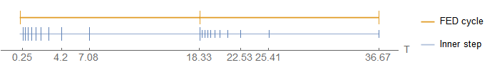
You can also think of this as breaking apart the proceeding in diffusion time into multiple blocks (= FED cycles). Each FED cycle has a fixed step size of \(\theta = \sum_{i=0}^{n-1}\tau_i\) and this size is the same for all cycles (like the usual step size in an explicit scheme). But each FED cycle is now divided into multiple inner steps (factors of \eqref{eq:FEDIntroduction_DiscreteDiffusion}) and each inner step has its own step size \(\tau_i\). Additionally, all FED cycles share the same inner steps, e.g. each cycle starts with an inner step with step size \(\tau_0\) and ends with \(\tau_{n-1}\). The following figure visualizes this for the previous example.
We have now seen how FED generally works. The next part focuses on simplifying the notation.
Matrix notation
Calculating FED like in the previous section may become unhandy for larger signals and/or larger filters. Luckily, there is an easier way to express the same logic using matrices. It turns out that this is also useful in generalising FED to arbitrary problems (as implied in the beginning).
The example so far is based on a PDE with some change of function value at each position over time. In \eqref{eq:FEDIntroduction_PDE} therefore the derivative definition depended on two variables. It is possible to transform the PDE to a system of ODEs by fixing space. The derivative can then be defined as
\begin{equation*} \frac{\mathrm{d} \fvec{u}(t)}{\mathrm{d} t} = A \cdot \fvec{u}(t). \end{equation*}Where \(\fvec{u}(t)\) is the vector containing the discrete set of spatial locations but which are still continuous in time \(t\). You can think of this as each vector component fixing some \(x\) position of the original continuous function \(u(x, t)\) but the function value of this position (e.g. the temperature value) still varies continuously over time. The benefit of this approach is that the operator \(\Delta\) is discarded and replaced by the matrix \(A \in \mathbb{R}^{N \times N}\) which returns us to \eqref{eq:FEDIntroduction_Arbitrary}. \(A\) is now responsible for approximating the second order derivative. To be consistent with \(\Delta\) it may be defined for the previous example as
\begin{equation*} A = \begin{pmatrix} -1 & 1 & 0 & 0 \\ 1 & -2 & 1 & 0 \\ 0 & 1 & -2 & 1 \\ 0 & 0 & 1 & -1 \\ \end{pmatrix}. \end{equation*}Note that the pattern encoded in this matrix is the same as in \eqref{eq:FEDIntroduction_Delta}: left and right neighbour weighted once and the centre value compensates for this. Hence, \(A \fvec{u}\) is the same as \(\Delta \fvec{u}\). By calculating
\begin{equation*} (I + \tau_1\cdot A) \fvec{u} = \begin{pmatrix} 1 & 0 & 0 & 0 \\ 0 & 1 & 0 & 0 \\ 0 & 0 & 1 & 0 \\ 0 & 0 & 0 & 1 \\ \end{pmatrix} \begin{pmatrix} 1 \\ 4 \\ 2 \\ 6 \\ \end{pmatrix} + \tau_1 \cdot \begin{pmatrix} -1 & 1 & 0 & 0 \\ 1 & -2 & 1 & 0 \\ 0 & 1 & -2 & 1 \\ 0 & 0 & 1 & -1 \\ \end{pmatrix} \begin{pmatrix} 1 \\ 4 \\ 2 \\ 6 \\ \end{pmatrix} = \begin{pmatrix} 2 \\ 2.33333 \\ 4 \\ 4.66667 \\ \end{pmatrix} \end{equation*}we obtain exactly the same result as in \eqref{eq:FEDIntroduction_ExampleFED}. A FED cycle with multiple iterations is done by repeatedly multiplying the brackets (cf. \eqref{eq:FEDIntroduction_Cycle})
\begin{equation*} \fvec{u}_{k+1} = \left( I + \tau_0 \cdot A \right) \left( I + \tau_1 \cdot A \right) \cdots \left( I + \tau_{n-1} \cdot A \right) \fvec{u}_k. \end{equation*}This is actually the basis to extend FED to arbitrary diffusion problems as denoted in \eqref{eq:FEDIntroduction_Arbitrary} [9-11]. The trick is to find an appropriate matrix \(A\). If you, for example, encode the local conductivity information, i.e. let \(A\) depend on the signal values: \(A(\fvec{u}_{k})\), it is possible to use FED for inhomogeneous diffusion problems.
In the next section, I want to give an overview of the relevant parameters when using FED.
Parameters
I already used some parameters, like \(\tau_{\text{max}}\), without explaining what they do. The following list contains all previously discussed parameters plus introducing new ones which were there only implicitly.
- \(T\): is the total diffusion time. A longer diffusion time means in general higher blurring of the signal. I already stated that the relation to the standard deviation is \(T = \frac{1}{2} \cdot \sigma\). Usually, the desired amount of blurring \(\sigma\) is given.
- \(M\): a new parameter denoting the number of FED cycles used. So far exactly one cycle was used in the examples but usually multiple cycles are desired. Since multiple cycles correspond to multiple filters applied to the signal and more filters mean a better Gaussian approximation, this parameter controls the quality. Larger \(M\) means better quality (better Gaussian approximation). This parameter must also be given.
- \(n\): is the length of one FED cycle, i.e. the number of iteration it contains. It corresponds to the length of an equivalent kernel with size \(2\cdot n + 1\). Usually, the total diffusion time \(T\) should be accomplished by \(M\) cycles of equal length. \(n\) is therefore the same for all cycles and can be calculated as [11] \begin{equation*} n = \left\lceil -\frac{1}{2} + \frac{1}{2} \cdot \sqrt{1 + \frac{12 \cdot T}{M \cdot \tau_{\text{max}}}} \right\rceil. \end{equation*}
- \(\theta\): a new parameter denoting the diffusion time for one FED cycle, i.e. how much further in time one cycle approaches. This is basically the sum of all steps \(\tau_i\) \begin{equation*} \theta = \sum_{i=0}^{n-1} \tau_i \end{equation*} but it is also possible to calculate it explicitly for a given kernel, e.g. for a box filter [10] \begin{equation*} \theta_{\text{box}}(n) = \tau_{\text{max}} \cdot \frac{n^2 + n}{3}. \end{equation*}
- \(\tau_{\text{max}}\): is the maximum possible time step from the Euler scheme which does not violate stability. It is defined by the stability region and is based on the eigenvalues of \(A\). More precisely, the relation [12] \begin{equation} \tau_{\text{max}} \leq \frac{1}{\left| \max_i{(\lambda_i)} \right|} \label{eq:FEDIntroduction_TauMax} \end{equation} for the eigenvalues \(\lambda_i\) must hold. It is possible to make a worst-case estimation of the eigenvalues with the Gershgorin circle theorem. This explains why \(\tau_{\text{max}} = \frac{1}{2}\) is used here: the largest eigenvalue of \(A\) is5 \(\lambda_{\text{max}} = 4\) and \(\frac{2}{4} = \frac{1}{2}\) is valid according to \eqref{eq:FEDIntroduction_TauMax}.
After giving an overview of the relevant parameters, I want to elaborate a little bit more on the relation between filters and FED.
Why box filters?
You may have noticed that I kind of silently used \eqref{eq:FEDIntroduction_Cycle} as a representation of a box filter. Actually, this is even more general since any symmetric filter with its coefficients summing up to 1 can be used. So, why using a box filter? Is the box filter not the filter with such a destructive behaviour in the frequency domain? You could argue that, but let me remind you that in FED we usually use several iterations (i.e. \(M>1\)) and therefore applying multiple box filters which behave more like a Gaussian filter in the end. But there are even better reasons to use a box filter here. They are best understood when looking at how other filters behave [6-8].
In what do varying filters differ? Most importantly, the varying time steps \(\tau_i\) used in \eqref{eq:FEDIntroduction_Cycle} depend on the concrete filter. The steps in \eqref{eq:FEDIntroduction_TimeStepsBox} e.g. correspond to a box filter. Other filters result in different step sizes [7]. If the \(\tau_i\) are different, also their sum \(\theta(n)\) is not the same for all filters. This means if we want to proceed with all filters a fixed amount of diffusion time per FED cycle, \(n\) must also be defined differently. Therefore, different filters result in different long iterations per FED cycle.
Three filters will now be analysed under two basic criteria:
- Quality: the general goal is to approximate a Gaussian function since this is what the (homogeneous) diffusion equation implies. So the question is: how well do multiple FED cycles approximate a Gaussian?
- Performance: it is good to have high quality but it must also be achieved in a reasonable amount of time. In terms of FED, performance is defined by \(n\), the number of iterations per cycle. As more iterations needed, as worse is the performance. So the question is: how many iterations are needed in total?
The test setup is now as follows: a total diffusion time of \(T=6\) should be achieved in \(M=3\) FED cycles to a signal of length 101 with a single peak in the middle
\begin{equation*} s(i) = \begin{cases} 1, & i = 51 \\ 0, & i \neq 51 \end{cases} \end{equation*}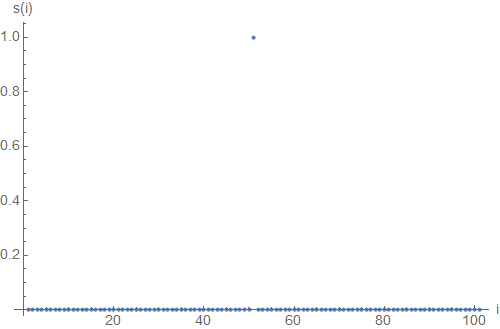
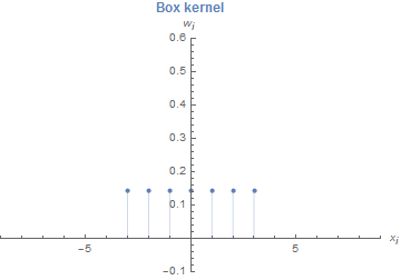
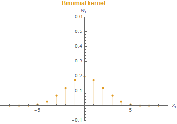
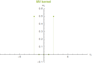
The behaviour of three different filters will now be analysed: box, binomial and the so-called maximum variance (MV) kernel. The first column of the following table shows a graph for each kernel (for concrete definition see [6]).
| Filter | Cycle time \(\theta(n)\) | Iterations \(n\) | Performance | Quality |
|---|---|---|---|---|
 |
\(\theta_{\text{box}}(n) = \frac{n^2+n}{6}\) | \(n_{\text{box}}=3\) | Good: \(\mathcal{O}_{\theta_{\text{box}}}(n^2)\) | Good |
 |
\(\theta_{\text{bin}}(n) = \frac{n}{4}\) | \(n_{\text{bin}}=8\) | Poor: \(\mathcal{O}_{\theta_{\text{bin}}}(n)\) | Very good |
 |
\(\theta_{\text{box}}(n) = \frac{n^2}{2}\) | \(n_{\text{MV}}=2\) | Very good: \(\mathcal{O}_{\theta_{\text{MV}}}(n^2)\) | Poor |
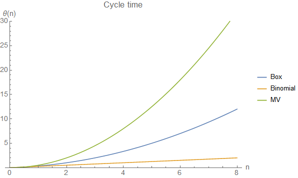
The second column shows the cycle time \(\theta(n)\) for each filter as a variable of \(n\). As faster this function growths as better because then the diffusion proceeds faster. The following figure shows how the MV kernel is superior in this task. But note also that the box filter, even though growing slower, increases still in a quadratic magnitude of \(n\) (hence \(\mathcal{O}_{\theta_{\text{box}}}(n^2)\) in the 4th column of the table).
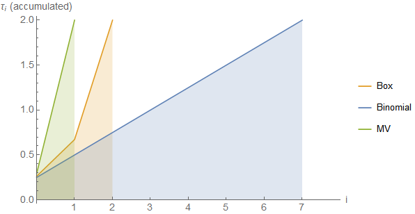
In the test scenario, each filter is supposed to make a total step of \(\frac{T}{M} = 2\), so \(n\) is adjusted for each filter in order to have proceeded the same diffusion time after each cycle. For the box filter, this leaves \(n_{\text{box}}=3\) since \(\frac{3^2 + 3}{6} = 2\). Therefore, over three iterations \(2 \cdot 3 = 6\) FED multiplications are necessary. Similarly for the other values in the third column. It is also worth looking how the time steps \(\tau_i\) accumulate over the multiplications (in only one FED cycle since the steps are equal among all cycles). The following figure shows how the \(\tau_i\) accumulate to 2 for each filter revealing that the MV kernel wins this race.
So far for on the performance point of view, but what are the results regarding approximation quality of a Gaussian? To answer this question an error value is calculated. More concretely, the total of absolute differences between the filter response and the corresponding Gaussian after each FED cycle is used
\begin{equation} E = \sum_{i=1}^{101} = \left| \operatorname{FED}_{T, \text{filter}}(s(i)) - G_{\sigma}(i) \right| \label{eq:FEDIntroduction_Error} \end{equation}where \(\operatorname{FED}_{T, \text{filter}}(s(i))\) denotes the result after applying the FED cycle for the specific filter up to the total diffusion time \(T\) and \(G_{\sigma}(i)\) is the Gaussian with the same standard deviation and mean as the filter response data.
Each of the filters is now applied three times to \(s(i)\) by using three FED cycles. Since the signal is just defined as a single peak of energy 1, the first iteration will produce the filter itself in each case.
Even though it is visible that all tend to take the shape of a Gaussian, it is also clear that the binomial filter performs best on this task. The visual representation together with the error value now also explains the fifth column of the table.
Summarising, we can now see that no filter is perfect in both disciplines. But if we would need to choose one filter, we would probably select the box filter. It offers reasonably approximation quality and still good performance and this is exactly the reason why in FED the cycle times resulting from the box filter are used.
As a last note, let me show how the step sizes \(\tau_i\) behave for larger \(n\). The following figure shows the individual step sizes \(\tau_i\) and their cumulative sum
\begin{equation*} \sum_{j=0}^{i} \tau_j \end{equation*}for \(n=50\). With higher cycle lengths the steps get even larger [12].
As you can see, in higher iterations the step sizes get larger and larger resulting in a great speedup (comparison between using a fixed time step of 0.5 and using the varying step sizes). What is more, there are many steps which actually exceed the stability limit from the explicit scheme. It can be shown though that at the end of a full cycle the result stays stable [10].
List of attached files:
- FEDIntroduction.nb [PDF] (Mathematica notebook containing the basic example of how to use FED)
- FEDIntroduction_Filters.nb [PDF] (Mathematica notebook with the analysation of the different filters)