When we are confronted with a new dataset, it is often of interest to analyse the structure of the data and search for patterns. Are the data points organized into groups? How close are the groups together? Are there any other interesting structures? These questions are addressed in the cluster analysis field. It contains a collection of unsupervised algorithms (meaning that they don't rely on class labels) which try to find these patterns. As a result, each data point is assigned to a cluster.
In \(k\)-means clustering, we define the number of clusters \(k\) in advance and then search for \(k\) groups in the data. Heuristic algorithms exist to perform this task computational efficient even though there is no guarantee to find a global optimum. Hartigan's method is one algorithm of this family. It is not to be confused with Lloyd's algorithm which is the standard algorithm in \(k\)-means clustering and so popular that people often only talk about \(k\)-means and what they mean is that they apply Lloyd's algorithm to achieve a \(k\)-means clustering result.
Whatever algorithm is used, they all belong to the family of centroid-based clustering where we calculate a representative for each cluster based on the points which belong to it. It is a new data point which condenses the major information of the cluster and a common approach is to use the centre of gravity
\begin{equation*} c_j = \frac{1}{\left| C_j \right|} \sum_{\fvec{x} \in C_j} \fvec{x}. \end{equation*}\(C_j\) is the set with all data points which are assigned to the \(j\)-th cluster. Also, we need a measure which tells us how good our current clustering is in a single numerical value. It is common to use the variance of the current partition
\begin{equation*} D_{var}(\mathfrak{C}) = \sum_{j=1}^{\left|\mathfrak{C}\right|} \sum_{\fvec{x} \in C_j} \left\| \fvec{x} - \fvec{c}_j \right\|^2. \end{equation*}\( \mathfrak{C} = \left\{ C_1, C_2, \ldots \right\}\) denotes the set of all clusters. This basically calculates the squared Euclidean distance from each data point \(\fvec{x}\) to its assigned cluster centre \(\fvec{c}_j\) and this over all clusters. As lower the value of \(D_{var}(\mathfrak{C})\), as less variance there is inside the clusters meaning that the data points are closer together. Usually, this is what we want. Hence, the \(k\)-means clustering algorithms try to minimize \(D_{var}(\mathfrak{C})\) but since they only work in a heuristic fashion, we can only end up in a local minimum.
Here, Hartigan's method is of interest. The underlying idea is sometimes also known as exchange clustering algorithm: start with an arbitrary initial clustering and then iterate over each data point. When doing so, re-assign the point to a different cluster on a trial basis and if this move improves \(D_{var}(\mathfrak{C})\), then accept the exchange; otherwise, when \(D_{var}(\mathfrak{C})\) gets worse, reject the exchange and revert it. For example, let's say that the data point \(\fvec{x}\) belongs initially to the cluster \(C_1\). We then remove it from \(C_1\) and add it to the set \(C_2\). After re-calculating \(D_{var}(\mathfrak{C})\) (the partition changed so it is likely that the variance changed as well), we decide if we keep the exchange or not. Summarizing, we apply the following steps:
- \(t=0.25\): select a new point which should be tested.
- \(t=0.5\): move the data point to a different cluster on a trial basis.
- \(t=0.75\): calculate the variance after the exchange is performed. This also means that, for the calculation of the variance, the new cluster centres are used (the ones which arise due to the exchange). If the variance is lower than before, we keep the change. Otherwise, it is reverted.
- \(t=1\): show the result after the data point is processed. The data point either keeps its old label (if the exchange resulted in no improvement of variance) or takes over the new label of the other cluster (if the exchange did result in an improvement).
The following animation shows an example for a two-dimensional dataset with the initial clustering
\begin{align} \begin{split} C_1 &= \{ (1, 1), (3, 3), (2, 2) \} \\ C_2 &= \{ (2, 1), (0, 2), (3, 5), (4, 4), (5,4) \}. \end{split} \label{eq:ExchangeClusteringAlgorithm_Dataset} \end{align}It shows each of the above-mentioned steps in increments of \(\Delta t = 0.25\). The algorithm runs two times over the complete dataset \(X = C_1 \cup C_2 \) and in every run each point is processed in the order shown in the animation (the order matters since a previous exchange can influence whether a later exchange is good or not since the cluster centres are re-calculated after each performed exchange). For this example, already in the second run there is no change and the algorithm converged (local minimum of \(D_{var}(\mathfrak{C})\) found).
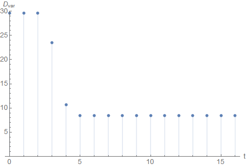
If we plot the variance \(D_{var}(\mathfrak{C})\) over the iteration time \(t\), we see that the algorithm converged at around \(t=5\).
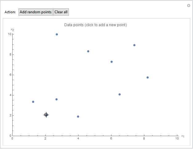
Maybe you want to explore Hartigan's method on a different dataset. For this purpose, you can use the general Mathematica notebook. Here, you can manually create your own dataset and then apply the algorithm from above.
List of attached files:
- ExchangeClusteringAlgorithm_General.nb [PDF] (Mathematica notebook with the general implementation of the algorithm and where you can create your own dataset)
- ExchangeClusteringAlgorithm_Manual.nb [PDF] (Mathematica notebook which goes through the above example step-by-step)
- ExchangeClusteringAlgorithm_Functions.nb [PDF] (Mathematica notebook with auxiliary functions used by the two other notebooks. Note that all notebooks must be stored in the same folder when executing)
← Back to the overview page