Estimate eigenvalues with the Gershgorin circle theorem


Eigenvalues are properly one of the most important metrics which can be extracted from matrices. Together with their corresponding eigenvector, they form the fundamental basis for many applications. Calculating eigenvalues from a given matrix is straightforward and implementations exist in many libraries. But sometimes the concrete matrix is not known in advance, e.g. when the matrix values are based on some bounded input data. In this case, it may be good to give at least some estimation of the range in which the eigenvalues can lie. As the name of this article suggests, there is a theorem intended for this use case and which will be discussed here.

What it does

For a square \( n \times n\) matrix \(A\) the Gershgorin circle theorem returns a range in which the eigenvalues must lie by simply using the information from the rows of \(A\). Before looking into the theorem though, let me remind the reader that eigenvalues may be complex valued (even for a matrix which contains only real numbers). Therefore, the estimation lives in the complex plane, meaning we can visualize the estimation in a 2D coordinate system with the real part as \(x\)- and the imaginary part as the \(y\)-axis. Note also that \(A\) has a maximum of \(n\) distinct eigenvalues.

For the theorem, the concept of a Gershgorin disc is relevant. Such a disk exists for each row of \(A\), is centred around the diagonal element \(a_{ii}\) (which may be complex as well) and the sum of the other elements in the row \(r_i\) constraint the radius. The disk is therefore defined as

\begin{equation} \label{eq:GershgorinCircle_Disc} C_i = \left\{c \in \mathbb{C} : \left| c - a_{ii} \right| \leq r_i\right\} \end{equation}

with the corresponding row sum

\begin{equation} \label{eq:GershgorinCircle_Disc_RowSum} r_i = \sum_{j=1,\\ j\not=i}^n \left|a_{ij}\right| \end{equation}

(absolute sum of all row values except the diagonal elements itself). As an example, let's take the following definition for

\begin{equation*} A = \begin{pmatrix} 4 & 3 & 15 \\ 1 & 1+i & 5 \\ -8 & -2 & 22 \end{pmatrix}. \end{equation*}

There are three Gershgorin discs in this matrix:

  • \(C_1\) with the centre point \(a_{11} = 4\) and radius \(r_1 = \left|3\right| + \left|15\right| = 18\)
  • \(C_2\) with the centre point \(a_{22} = 1+i\) and radius \(r_2 = \left|1\right| + \left|5\right| = 6\)
  • \(C_3\) with the centre point \(a_{33} = 22\) and radius \(r_3 = \left|-8\right| + \left|-2\right| = 10\)

We have now all ingredients for the statement of the theorem:

Definition 1: Gershgorin circle theorem

Every eigenvalue \(\lambda \in \mathbb{C}\) of a square matrix \(A \in \mathbb{R}^{n \times n}\) lies in at least one of the Gershgorin discs \(C_i\) (\eqref{eq:GershgorinCircle_Disc}). The possible range of the eigenvalues is defined by the outer borders of the union of all discs

\begin{equation*} C = \bigcup_{i=1}^{n} C_i. \end{equation*}

The union, in the case of the example, is \(C = C_1 \cup C_2 \cup C_3\) and based on the previous information of the discs we can now visualize the situation in the complex plane. In the following figure, the discs are shown together with their disc centres and the actual eigenvalues (which are all complex in this case)

\begin{equation*} \lambda_1 = 13.4811 - 7.48329 i, \quad \lambda_2 = 13.3749 + 7.60805 i \quad \text{and} \quad \lambda_3 = 0.14402 + 0.875241 i. \end{equation*}

Figure 1: The three Gershgorin discs of the matrix \(A\) together with eigenvalues \(\lambda_i\) (green). The disc centres \(a_{ii}\) are shown in red. E.g. for \(C_2\) a disc around the point \((\operatorname{Re}(a_{22}), \operatorname{Im}(a_{22})) = (1, 1)\) with radius \(r_2 = 6\) is drawn. Markers show the label for the disc centres and eigenvalues. The rectangle is a rough estimation of the possible range where the eigenvalues lie (see below).

Indeed, all eigenvalues lie in the blue area defined by the discs. But you also see from this example that not all discs have to contain an eigenvalue (the theorem does not state that each disc has one eigenvalue). E.g. \(C_3\) on the right side does not contain any eigenvalue. This is why the theorem makes only a statement about the complete union and not each disc independently. Additionally, you can also see that one disc can be completely contained inside another disc as it is the case with \(C_2\) which lies inside \(C_1\). In this case, \(C_2\) does not give any useful information at all, since it does not expand the union \(C\) (if \(C_2\) would be missing, nothing changes regarding the complete union of all discs, i.e. \(C=C_1 \cup C_2 \cup C_3 = C_1 \cup C_3\)).

If we want to estimate the range in which the eigenvalues of \(A\) will lie, we can use the extrema values from the union, e.g.

\begin{equation*} \left[4-18; 22+10\right]_{\operatorname{Re}} = \left[-14; 32\right]_{\operatorname{Re}} \quad \text{and} \quad \left[0 - 18; 0 + 18\right]_{\operatorname{Im}} = \left[-18; 18 \right]_{\operatorname{Im}} \end{equation*}

for the real and complex range respectively. This defines nothing else than a rectangle containing all discs. Of course, the rectangle is an even more inaccurate estimation as the discs already are, but the ranges are easier to handle (e.g. to decide if a given point lies inside the valid range or not). Furthermore, if we have more information about the matrix, like that it is symmetric and real-valued and therefore contains only real eigenvalues, we can discard the complex range completely.

In summary, with the help of the Gershgorin circle theorem, it is very easy to give an estimation of the eigenvalues of some matrix. We only need to look at the diagonal elements and corresponding sum of the rest of the row and get a first estimate of the possible range. In the next part, I want to discuss why this estimation is indeed correct.

Why it works

Let's start again with a 3-by-3 matrix called \(B\) but now I want to use arbitrary coefficients

\begin{equation*} B = \begin{pmatrix} b_{11} & b_{12} & b_{13} \\ b_{21} & b_{22} & b_{23} \\ b_{31} & b_{32} & b_{33} \end{pmatrix}. \end{equation*}

Any eigenvalue \(\lambda\) with corresponding eigenvector \(\fvec{u} = (u_1,u_2,u_3)^T\) for this matrix is defined as

\begin{align*} B\fvec{u} &= \lambda \fvec{u} \\ \begin{pmatrix} b_{11} & b_{12} & b_{13} \\ b_{21} & b_{22} & b_{23} \\ b_{31} & b_{32} & b_{33} \end{pmatrix} \begin{pmatrix} u_{1} \\ u_{2} \\ u_{3} \end{pmatrix} &= \lambda \begin{pmatrix} u_{1} \\ u_{2} \\ u_{3} \end{pmatrix} \end{align*}

Next, see how the equation for each component of \(\fvec{u}\) looks like. I select \(u_1\) and also assume that this is the largest absolute1 component of \(\fvec{u}\), i.e. \(\max_i{\left|u_i\right|} = \left|u_1\right|\). This is a valid assumption since one component must be the maximum and there is no restriction on the component number to choose for the next discussion. For \(u_1\) it results in the following equation which will be directly transformed a bit

\begin{align*} b_{11}u_1 + b_{12}u_2 + b_{13}u_3 &= \lambda u_1 \\ b_{12}u_2 + b_{13}u_3 &= \lambda u_1 - b_{11}u_1 \\ \left| u_1 (\lambda - b_{11}) \right| &= \left| b_{12}u_2 + b_{13}u_3 \right| \\ \end{align*}

All \(u_1\) parts are placed on one side together with the diagonal element and I am only interested in the absolute value. For the right side, there is an estimation possible

\begin{equation*} \left| b_{12}u_2 + b_{13}u_3 \right| \leq \left| b_{12}u_2 \right| + \left| b_{13}u_3 \right| \leq \left| b_{12}u_1 \right| + \left| b_{13}u_1 \right| = \left| b_{12} \right| \left| u_1 \right| + \left| b_{13} \right| \left| u_1 \right| \end{equation*}

First, two approximations: with the help of the triangle inequality for the \(L_1\) norm2 and with the assumption that \(u_1\) is the largest component. Last but not least, the product is split up. In short, this results to

\begin{align*} \left| u_1 \right| \left| (\lambda - b_{11}) \right| &\leq \left| b_{12} \right| \left| u_1 \right| + \left| b_{13} \right| \left| u_1 \right| \\ \left| \lambda - b_{11} \right| &\leq \left| b_{12} \right| + \left| b_{13} \right| \\ \left| \lambda - b_{11} \right| &\leq r_1 \\ \end{align*}

where \(\left| u_1 \right|\) is thrown away completely. This states that the eigenvalue \(\lambda\) lies in the radius of \(r_1\) (cf. \eqref{eq:GershgorinCircle_Disc_RowSum}) around \(b_{11}\) (the diagonal element!). For complex values, this defines the previously discussed discs.

Two notes on this insight:

  • The result is only valid for the maximum component of the eigenvector. Note also that we usually don't know which component of the eigenvector is the maximum (if we would now, we probably don't need to estimate the eigenvalues in the first place because we already have them).
  • In the explanation above only one eigenvector was considered. But usually, there are more (e.g. usually three in the case of matrix \(B\)). The result is therefore true for each maximum component of each eigenvector.

This also implies that not every eigenvector gives new information. It may be possible that for multiple eigenvectors the first component is the maximum. In this case, one eigenvector would have been sufficient. As an example, let's look at the eigenvectors of \(A\). Their absolute value is defined as (maximum component highlighted)

\begin{equation*} \left| \fvec{u}_1 \right| = \begin{pmatrix} {\color{Aquamarine}1.31711} \\ 0.40112 \\ 1 \end{pmatrix}, \quad \left| \fvec{u}_2 \right| = \begin{pmatrix} {\color{Aquamarine}1.33013} \\ 0.431734 \\ 1 \end{pmatrix} \quad \text{and} \quad \left| \fvec{u}_3 \right| = \begin{pmatrix} 5.83598 \\ {\color{Aquamarine}12.4986} \\ 1 \end{pmatrix}. \end{equation*}

As you can see, the third component is never the maximum. But this is coherent to the example from above: the third disc \(C_3\) did not contain any eigenvalue.

What the theorem now does is some kind of worst-case estimate. We now know that if one component of some eigenvector is the maximum, the row corresponding to this component defines a range in which the eigenvalue must lie. But since we don't know which component will be the maximum the best thing we can do is to assume that every component was the maximum in some eigenvector. In this case, we need to consider all diagonal elements and their corresponding absolute sum of the rest of the row. This is exactly what is done in the example from above. There is another nice feature which can be derived from the theorem when we have disjoint discs. This will be discussed in the next section.

The story about disjoint discs

Additional statements can be extracted from the theorem when we deal with disjoint disc areas3. Consider another example with the following matrix

\begin{equation*} D= \begin{pmatrix} 1 & -2 & 3 \\ 0 & 6 & 1 \\ 3 & 0 & 9+10 i \\ \end{pmatrix}. \end{equation*}

Using Geshgorin discs this results in a situation like shown in the following figure.


Figure 2: Gershgorin discs for the matrix \(D\). Markers show the label for the disc centres and eigenvalues.

This time we have one disc (centred at \(d_{33}=9+10i\)) which does not share a common area with the other discs. With other words: we have two disjoint areas. The question is: does this gives us additional information?. Indeed, it is possible to state that there is exactly one eigenvalue in the third disc.

Definition 2: Gershgorin circle theorem with disjoint discs

Let \(A \in \mathbb{R}^{n \times n}\) be a square matrix with \(n\) Gershgorin discs (\eqref{eq:GershgorinCircle_Disc}). Then, each joined area defined by the discs contains so many eigenvalues as discs contributed to the area. If the set \(\tilde{C}\) contains \(k\) discs which are disjoint from the other \(n-k\) discs, then \(k\) eigenvalues lie in the range defined by the union

\begin{equation*} \bigcup_{C \in \tilde{C}} C \end{equation*}

of the discs in \(\tilde{C}\).

In the example, we have exactly one eigenvalue in the third disc and exactly two eigenvalues somewhere in the union of disc one and two4. Why is it possible to restrict the estimation when we deal with disjoint discs? To see this, let me first remind you that the eigenvalues of any diagonal matrix are exactly the diagonal elements itself. Next, I want to define a new function which separates the diagonal elements from the off-diagonals

\begin{align*} \tilde{D}(\alpha) &= \begin{pmatrix} 1 & 0 & 0 \\ 0 & 6 & 0 \\ 0 & 0 & 9+10 i \end{pmatrix} + \alpha \begin{pmatrix} 0 & -2 & 3 \\ 0 & 0 & 1 \\ 3 & 0 & 0 \end{pmatrix} \\ \tilde{D}(\alpha) &= D_1 + \alpha D_2 \end{align*}

With \(\alpha \in [0;1]\) this smoothly adds the off-diagonal elements in \(D_2\) to the matrix \(D_1\) containing only the diagonal elements by starting from \(\tilde{D}(0) = \operatorname{diag}(D) = D_1\) and ending at \(\tilde{D}(1) = D_1 + D_2 = D\). Before we see why this step is important, let us first consider the same technique for a general 2-by-2 matrix

\begin{align*} F &= \begin{pmatrix} f_{11} & f_{12} \\ f_{21} & f_{22} \end{pmatrix} \\ \Rightarrow \tilde{F}(\alpha) &= F_1 + \alpha F_2 \end{align*}

If we now want to calculate the eigenvalues for \(\tilde{F}\), we need to find the roots of the corresponding characteristic polynomial, meaning

\begin{align*} \left| \tilde{F} - \lambda I \right| &= 0 \\ \left| F_1 + \alpha F_2 - \lambda I \right| &= 0 \\ \left| \begin{pmatrix} f_{11} & 0 \\ 0 & f_{22} \end{pmatrix} + \alpha \begin{pmatrix} 0 & f_{12} \\ f_{21} & 0 \end{pmatrix} - \lambda \begin{pmatrix} 1 & 0 \\ 0 & 1 \end{pmatrix} \right| &= 0. \end{align*}

The solution for the first root of this polynomial and therefore the first eigenvalue is defined as

\begin{equation*} \lambda(\alpha) = \frac{1}{2} \left(-\sqrt{{\color{Aquamarine}4 \alpha ^2 f_{12} f_{21}} +f_{11}^2+f_{22}^2-2 f_{11} f_{22}}+f_{11}+f_{22}\right). \end{equation*}

The thing I am driving at is the fact that the eigenvalue \(\lambda(\alpha)\) changes only continuously with increasing value of \(\alpha\) (highlighted position) and as closer \(\alpha\) gets to 1 as more off-diagonals are added. Especially, \(\lambda(\alpha)\) does not jump suddenly somewhere completely different. I chose a 2-by-2 matrix because this point is easier to see here. Finding roots of higher dimensional matrices can suddenly become much more complicated. But the statement of continuously increasing eigenvalues stays true, even for matrices with higher dimensions.

No back to the matrix \(\tilde{D}(\alpha)\) from the example. We will now increase \(\alpha\) and see how this affects our discs. The principle is simple: just add both matrices together and apply the circle theorem on the resulting matrix. The following animation lets you perform the increase of \(\alpha\).


Figure 3: Increase of \(\alpha\) for the matrix \(\tilde{D}(\alpha)\) showing how the eigenvalues smoothly leave the initial disc centres. Markers show the label for the disc centres and eigenvalues.

As you can see, the eigenvalues start at the disc centres because here only the diagonal elements remain, i.e. \(\tilde{D}(0) = D_1\). With increasing value of \(\alpha\) more and more off-diagonal elements are added letting the eigenvalues move away from the centre. But note again that this transition is smooth: no eigenvalue suddenly jumps to a completely different position. Note also that at some point the discs for the first and second eigenvalue merge together.

Now the extended theorem becomes clear: if the eigenvalues start at the disc centres, don't jump around and if the discs don't merge at \(\alpha=1\), then each union must contain as many eigenvalues as discs contributed to this union. In the example, this gives us the proof that \(\lambda_3\) must indeed lie in the disc around \(d_{33}\).

List of attached files:


1. The absolute value is necessary here because the components may be complex.
2. For two vectors \(\fvec{x}\) and \(\fvec{y}\) the inequality \(\left\| \fvec{x} + \fvec{y} \right\| \leq \left\| \fvec{x} \right\| + \left\| \fvec{y} \right\|\) holds (in this case \(\left\|\cdot\right\|_1\)). Intuitively, this means that the way over a detour is always longer or equal to the direct way.
3. The following discussion is based on the statements of these slides.
4. To apply the notation of the theorem to the example, \(\tilde{C}\) could be defined as \(\tilde{C} = \{C_1, C_2\}\) and the set of other \(n-k\) discs contains only the disc \(C_3\). But defining it the other way around, \(\tilde{C} = \{C_3\}\), is also possible (and doesn't matter).

Intersection area of two circles with implementation in C++


In this article, I want to discuss how the intersection area of two circles can be calculated. Given are only the two circles with their corresponding centre point together with the radius and the result is the area which both circles share in common. First, I want to take a look at how the intersection area can be calculated and then how the needed variables are derived from the given data. At the end of the article, I supply running code in C++.

The following figure illustrates the general problem. A small and a large circle is shown and both share a common area at the right part of the first circle.

Two circles which intersect and share a common area (angle < 180°)
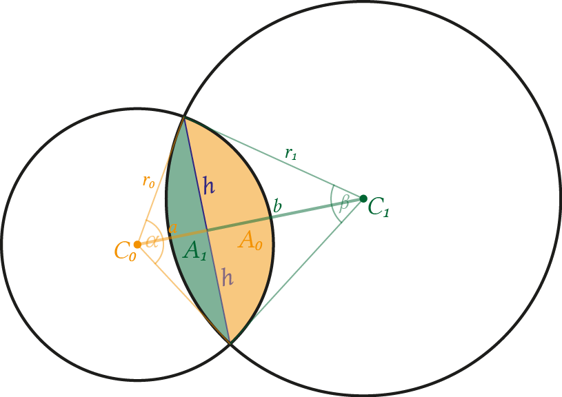
Figure 1: Geometry for two circular segments of two intersecting circles used to calculate the intersection area.

As the figure already depicts, the problem is solved by calculating the area of the two circular segments formed by the two circles. The total intersecting area is then simply

\begin{equation*} A_0 + A_1. \end{equation*}

As equation 15 from MathWorld shows, the area of one circular segment is calculated as (all angles are in radiant)

\begin{equation*} \begin{split} A &= \frac{1}{2} r^2 (\theta - \sin(\theta)), \\ &= \frac{1}{2} r^2 \theta - \frac{1}{2} r^2 \sin(\theta). \end{split} \end{equation*}

The formula consists of two parts. The left part is the formula for the area of the circular sector (complete wedge limited by the radius), which is similar to the formula of the complete circle area (\( r^2\pi \)) where the arc length takes a complete round of the circle. Here instead, the arc length is explicitly specified by \(\theta\) instead of \(\pi\). If you plug a complete round into \(\theta\), you get the same result: \( \frac{1}{2} r^2 2\pi = r^2\pi \). The right part calculates the area of the isosceles triangle (triangle with the radii as sides and heights as baseline), which is a little bit harder to see. With the double-angle formula

\begin{equation*} \sin(2x) = 2\sin(x)\cos(y) \end{equation*}

\(\sin(\theta)\) can be rewritten as

\begin{equation*} \sin(\theta) = 2\sin\left(\frac{1}{2}\theta\right) \cos\left(\frac{1}{2}\theta\right). \end{equation*}

This leaves for the right part of the above formula

\begin{equation*} \frac{1}{2} r^2 \sin(\theta) = r^2 \sin\left(\frac{1}{2}\theta\right) \cos\left(\frac{1}{2}\theta\right). \end{equation*}

Also, note that \(r \sin\left(\frac{1}{2}\theta\right) = a\) and \( r \cos\left(\frac{1}{2}\theta\right) = h\) (imagine the angle \(\frac{\alpha}{2}\) from the above figure in a unit circle), which results in

\begin{equation*} r^2 \sin\left(\frac{1}{2}\theta\right) \cos\left(\frac{1}{2}\theta\right) = ar \end{equation*}

and since we have an isosceles triangle, this is exactly the area of the triangle.

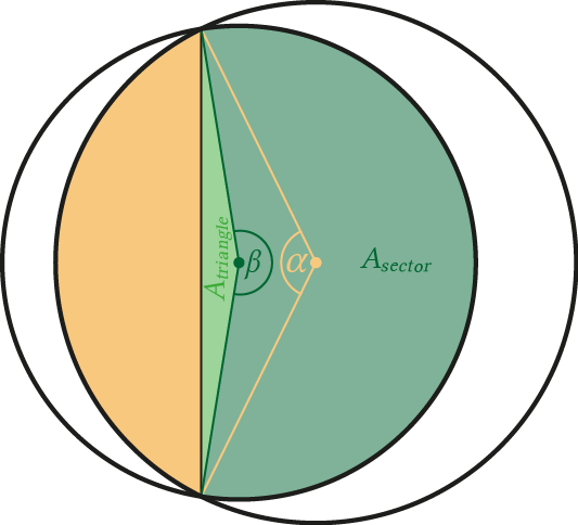
Originally, the formula is only defined for angles \(\theta < \pi\) (and probably \(\theta \geq 0\)). In this case, \(\sin(\theta)\) is non-negative and the area of the circular segment is the subtraction of the triangle area from the circular sector area (\( A = A_{sector} - A_{triangle} \)). But as far as I can see, this formula also works for \(\theta \geq \pi\), if the angle stays in the range \([0;2\pi]\). In this case, the triangle area and the area of the circular sector need to get added up (\( A = A_{sector} + A_{triangle} \)), which is considered in the formula by a negative \(\sin(\theta)\) (note the negative factor before the \(\sin(\theta)\) function). The next figure also depicts this situation.

Two circles which intersect and share a common area
Figure 2: Circular segments of two intersecting circles with a central angle \(\beta \geq \pi\).

The following table gives a small example of these two elementary cases (circular sector for one circle).

\(r\) \(\theta\) \(a = \frac{1}{2} r^2 \theta\) \(b = \frac{1}{2} r^2 \sin(\theta)\) \(A = a - b\)
\(2\) \(\frac{\pi}{3} = 60°\) \(\frac{2 \pi }{3}\) \(\sqrt{3}\) \(\frac{2 \pi }{3} - \sqrt{3} = 0.362344\)
\(2\) \(\frac{4\pi}{3} = 240°\) \(\frac{8 \pi }{3}\) \(-\sqrt{3}\) \(\frac{8 \pi }{3}- (-\sqrt{3}) = 10.1096\)

It is also from interest to see the area of the circular segment as a function of \(\theta\):

Graph of one circular segment area as a function of theta
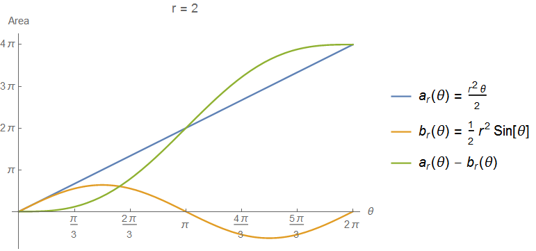
Figure 3: Area of one circular segment as a function of \(\theta\) build upon the area of the circular sector \(A_{sector} = a_r(\theta)\) and the area of the triangle \(A_{triangle} = \left| b_r(\theta) \right|\) (Mathematica Notebook).

It is noticeable that the area of one circular segment (green line) starts degressively from the case where the two circles just touch each other, because here the area of the triangle is subtracted. Beginning from the middle at \(\theta = \pi\) the area of the triangle gets added and the green line proceeds progressively until the two circles contain each other completely (full circle area \(2^2\pi=4\pi\)). Of course, the function itself is independent of any intersecting scenario (it gives just the area for a circular segment), but the interpretation fits to our intersecting problem (remember that in total areas of two circular segments will get added up).

Next, we want to use the formula. The radius \(r\) of the circle is known, but we need to calculate the angle \(\theta\). Let's start with the first circle. The second then follows easily. With the notation from the figure, we need the angle \(\alpha\). Using trigonometric functions, this can be done by

\begin{equation*} \begin{split} \tan{\frac{\alpha}{2}} &= \frac{\text{opposite}}{\text{adjacent}} = \frac{h}{a} \\ \text{atan2}(y, x) &= \text{atan2}(h, a) = \frac{\alpha}{2} \end{split} \end{equation*}

The \(\text{atan2}(y, x)\) function is the extended version of the \(\tan^{-1}(x)\) function where the sign of the two arguments is used to determine a resulting angle in the range \([-\pi;\pi]\). Please note that the \(y\) argument is passed first. This is common in many implementations, like also in the here used version of the C++ standard library std::atan2(double y, double x). For the intersection area the angle should be be positive and in the range \([0;2\pi]\) as discussed before, so in total we have

\begin{equation*} \alpha = \text{atan2}(h, a) \cdot 2 + 2 \pi \mod 2 \pi. \end{equation*}

Firstly, the range is expanded to \([-2\pi;2\pi]\) (factor from the previous equation, since the height \(h\) covers only half of the triangle). Secondly, positivity is ensured by adding \(+2\pi\) leaving a resulting interval of \([0;4\pi]\). Thirdly, the interval is shrinked to \([0;2\pi]\) to stay inside one circle round.

Before we can calculate the \(\alpha\) angle, we need to find \(a\) and \(h\)1. Let's start with \(a\). The two circles build two triangles (not to be confused with the previous triangle used to calculate the area of the circular segment) with the total baseline \(d=a+b = \left\| C_0 - C_1 \right\|_2 \) and the radii (\(r_0,r_1\)) as sides, which give us two equations

\begin{equation*} \begin{split} r_0^2 &= a^2 + h^2, \\ r_1^2 &= b^2 + h^2. \end{split} \end{equation*}

The parameter \(b\) in the second equation can be omitted (using \(d-a=b\))

\begin{equation*} r_1^2 = b^2 + h^2 = (d-a)^2 + h^2 = d^2 - 2da + a^2 + h^2 \end{equation*}

and the equation solved by \(h^2\)

\begin{equation*} h^2 = r_1^2 - d^2 + 2da - a^2. \end{equation*}

Plugging this into the equation for the first triangle

\begin{equation*} \begin{split} r_0^2 &= a^2 + r_1^2 - d^2 + 2da - a^2 \\ r_0^2 - r_1^2 + d^2 &= 2da \\ a &= \frac{r_0^2 - r_1^2 + d^2}{2d} \end{split} \end{equation*}

results in the desired distance \(a\). This directly gives us the height

\begin{equation*} h = \sqrt{r_0^2 - a^2}. \end{equation*}

Using the existing information the angle \(\beta\) for the second circle can now easily be calculated

\begin{equation*} \beta = \text{atan2}(h, d-a) \cdot 2 + 2 \pi \mod 2 \pi. \end{equation*}

Now we have every parameter we need to use the area function and it is time to summarize the findings in some code.


/**
 * @brief Calculates the intersection area of two circles.
 *
 * @param center0 center point of the first circle
 * @param radius0 radius of the first circle
 * @param center1 center point of the second circle
 * @param radius1 radius of the second circle
 * @return intersection area (normally in px²)
 */
double intersectionAreaCircles(const cv::Point2d& center0, const double radius0, const cv::Point2d& center1, const double radius1)
{
	CV_Assert(radius0 >= 0 && radius1 >= 0);

	const double d_distance = cv::norm(center0 - center1);	// Euclidean distance between the two center points

	if (d_distance > radius0 + radius1)
	{
		/* Circles do not intersect */
		return 0.0;
	}

	if (d_distance <= fabs(radius0 - radius1)) // <= instead of <, because when the circles touch each other, it should be treated as inside
	{
		/* One circle is contained completely inside the other, just return the smaller circle area */
		const double A0 = PI * std::pow(radius0, 2);
		const double A1 = PI * std::pow(radius1, 2);

		return radius0 < radius1 ? A0 : A1;
	}

	if (d_distance == 0.0 && radius0 == radius1)
	{
		/* Both circles are equal, just return the circle area */
		return PI * std::pow(radius0, 2);
	}

	/* Calculate distances */
	const double a_distanceCenterFirst = (std::pow(radius0, 2) - std::pow(radius1, 2) + std::pow(d_distance, 2)) / (2 * d_distance); // First center point to the middle line
	const double b_distanceCenterSecond = d_distance - a_distanceCenterFirst;	// Second centre point to the middle line
	const double h_height = std::sqrt(std::pow(radius0, 2) - std::pow(a_distanceCenterFirst, 2));	// Half of the middle line

	/* Calculate angles */
	const double alpha = std::fmod(std::atan2(h_height, a_distanceCenterFirst) * 2.0 + 2 * PI, 2 * PI); // Central angle for the first circle
	const double beta = std::fmod(std::atan2(h_height, b_distanceCenterSecond) * 2.0 + 2 * PI, 2 * PI); // Central angle for the second circle

	/* Calculate areas */
	const double A0 = std::pow(radius0, 2) / 2.0 * (alpha - std::sin(alpha));	// Area of the first circula segment
	const double A1 = std::pow(radius1, 2) / 2.0 * (beta - std::sin(beta));		// Area of the second circula segment

	return A0 + A1;
}

Basically, the code is a direct implementation of the discussed points. The treatment of the three special cases (no intersection, circles completely inside each other, equal circles) are also from Paul Bourke's statements. Beside the functions of the C++ standard library I also use some OpenCV datatypes (the code is from a project which uses this library). But they play no important role here, so you can easily replace them with your own data structures.

I also have a small test method which covers four basic cases. The reference values are calculated in a Mathematica notebook.


void testIntersectionAreaCircles()
{
	/* Reference values from IntersectingCirclesArea_TestCases.nb */
	const double accuracy = 0.00001;
	CV_Assert(std::fabs(intersectionAreaCircles(cv::Point2d(200, 200), 100, cv::Point2d(300, 200), 120) - 16623.07332) < accuracy);	// Normal intersection
	CV_Assert(std::fabs(intersectionAreaCircles(cv::Point2d(200, 200), 100, cv::Point2d(220, 200), 120) - 31415.92654) < accuracy);	// Touch, inside
	CV_Assert(std::fabs(intersectionAreaCircles(cv::Point2d(200, 200), 100, cv::Point2d(400, 200), 100) - 0.0) < accuracy);			// Touch, outside
	CV_Assert(std::fabs(intersectionAreaCircles(cv::Point2d(180, 200), 100, cv::Point2d(220, 200), 120) - 28434.24854) < accuracy);	// Angle greater than 180°
}

List of attached files:


1. The derivations are based on the work by Paul Bourke.

Representation of a line in the polar coordinate system


Recently, I read a tutorial about Hough line transform at the OpenCV tutorials. It is a technique to find lines in an image using a parameter space. As explained in the tutorial, for this it is necessary to use the polar coordinate system. In the commonly used Cartesian coordinate system, a line would be represented by \(y=mx+b\). In the polar coordinate system on the other hand, a line is represented by

\begin{equation} y=-\frac{\cos{\theta}}{\sin{\theta}}x + \frac{\rho}{\sin{\theta}}. \label{eq:PolarCoordinateSystem_LineRepresentation} \end{equation}

This article tries to explain the relation between these two forms.

In \eqref{eq:PolarCoordinateSystem_LineRepresentation} there are two new parameters: radius \(\rho\) and angle \(\theta\) as also depicted in the following figure. \(\rho\) is the length of a vector which always starts at the pole \((0,0)\) (analogous term to the origin in the Cartesian coordinate system) and ends at the line (orange in the figure) so that \(\rho\) will be orthogonal to the line. This is important because otherwise the following conclusions wouldn't work.

Illustration of the line polar coordinate system
Figure 1: Illustration of a line in the polar coordinate system with the radius \(\rho\) and angle \(\theta\).

So, first start with the \(y\)-intercept \(b=\frac{\rho}{\sin{\theta}}\). Note that the angle \(\theta\) comes up twice: between the \(x\)-axis and the \(\rho\) vector plus between the \(y\)-axis and the blue line (on the right side). We will use trigonometrical functions to calculate the \(y\)-intercept. This is simply done by using the \(\sin\)-function

\begin{equation*} \begin{split} \sin{\theta} &= \frac{\text{opposite}}{\text{hypotenuse}} \\ \sin{\theta} &= \frac{\rho}{b} \\ b &= \frac{\rho}{\sin{\theta}} \end{split} \end{equation*}

and that is exactly what the equation said for the \(y\)-intercept.

Now it is time for the slope \(m=-\frac{\cos{\theta}}{\sin{\theta}}\). For this, the relation

\begin{equation*} m = \tan{\alpha} \end{equation*}

is needed, where \(\alpha\) is the slope angle of the line. \(\alpha\) can be calculated by using our known \(\theta\) angle:

\begin{equation*} \alpha = 180^{\circ} - (180^{\circ} - 90^{\circ} - \theta) = 90^{\circ} + \theta. \end{equation*}

Now we have \(m=\tan{\left(90^{\circ} + \theta\right)}\), which is equivalent to \(m=\frac{\sin{\left(90^{\circ} + \theta\right)}}{\cos{\left(90^{\circ} + \theta\right)}}\). Because of \(\sin{x}=\cos{\left(90^{\circ}-x\right)}\) and \(\cos{x}=\sin{\left(90^{\circ}-x\right)}\) we can do a little bit of rewriting

\begin{equation*} m=\frac {\cos\left({90^{\circ} - (90^{\circ} + \theta)}\right)} {\sin\left({90^{\circ} - (90^{\circ} + \theta}\right))} = \frac {\cos\left({-\theta}\right)} {\sin\left({-\theta}\right)} = \frac {\cos\left({\theta}\right)} {-\sin\left({\theta}\right)} = -\frac {\cos\left({\theta}\right)} {\sin\left({\theta}\right)} \end{equation*}

and we have exactly the form we need. In the last step, I used the property that \(\sin(x) = -\sin(-x)\) is an odd and \(\cos(x) = \cos(-x)\) an even function.