This is the third part of a series consisting of three articles with the goal to introduce some general concepts and concrete algorithms in the field of neural network optimizers. As a reminder, here is the table of contents:
We covered two important concepts of optimizers in the previous sections, namely the introduction of a momentum term and adaptive learning rates. However, other variations, combinations or even additional concepts have also been proposed1.
Each optimizer has its own advantages and limitations making it suitable for specific contexts. It is beyond the scope of this series to name or introduce them all. Instead, we shortly explain the well established Adam optimizer as one example. It also re-uses some of the ideas discussed previously.
Before we proceed, we want to stress some thoughts regarding the combination of optimizers. One obvious choice might be to combine the momentum optimizer with the adaptive learning scheme. Even though this is theoretically possible and even an option in an implementation of the RMSProp algorithm, there might be a problem.
The main concept of the momentum optimizer is to accelerate when the direction of the gradient remains the same in subsequent iterations. As a result, the update vector increases in magnitude. This, however, contradicts one of the goals of adaptive learning rates which tries to keep the gradients in “reasonable ranges”. This may lead to issues when the momentum vector \(\fvec{m}\) increases but then gets scaled down again by the scaling vector \(\fvec{s}\).
It is also noted by the authors of RMSProp that the direct combination of adaptive learning rates with a momentum term does not work so well. The theoretical argument discussed might be a cause for these observations.
In the following, we first define the Adam algorithm and then look at the differences compared to previous approaches. The first is the usage of first-order moments which behave differently compared to a momentum vector. We are using an example to see how this choice has an advantage in skipping suboptimal local minima. The second difference is the usage of bias-correction terms necessary due to the zero-initialization of the moment vectors. Finally, we are also going to take a look at different trajectories.
This optimizer was introduced by Diederik P. Kingma and Jimmy Ba in 2017. It mainly builds upon the ideas from AdaGrad and RMSProp, i.e. adaptive learning rates, and extends these approaches. The name is derived from adaptive moment estimation.
Additionally to the variables used in classical gradient descent, let \(\fvec{m} = (m_1, m_2, \ldots, m_n) \in \mathbb{R}^n\) and \(\fvec{s} = (s_1, s_2, \ldots, s_n) \in \mathbb{R}^n\) be the vectors with the estimates of the first and second raw moments of the gradients (same lengths as the weight vector \(\fvec{w}\)). Both vectors are initialized to zero, i.e. \(\fvec{m}(0) = \fvec{0}\) and \(\fvec{s}(0) = \fvec{0}\). The hyperparameters \(\beta_1, \beta_2 \in [0;1[\) denote the decaying rates for the moment estimates and \(\varepsilon \in \mathbb{R}^+\) is a smoothing term. Then, the Adam optimizer defines the update rules
to find a path from the initial position \(\fvec{w}(0)\) to a local minimum of the error function \(E\left(\fvec{w}\right)\). The symbol \(\odot\) denotes the point-wise multiplication and \(\oslash\) the point-wise division between vectors.
There is a very close relationship to adaptive learning rates. In fact, the update rule of \(\fvec{s}(t)\) in \eqref{eq:AdamOptimizer_Adam} is identical to the one in the adaptive learning scheme. We also see that there is an \(\fvec{m}\) vector, although this one is different compared to the one defined in momentum optimization. We are picking up this point shortly.
In the description of Adam, the arguments are more statistically-driven: \(\fvec{m}\) and \(\fvec{s}\) are interpreted as exponentially moving averages of the first and second raw moment of the gradient. That is, \(\fvec{m}\) is a biased estimate of the means of the gradients and \(\fvec{s}\) is a biased estimate of the uncentred variances of the gradients. In total, we can say that the Adam update process uses information about where the gradients are located on average and how they tend to scatter.
In momentum optimization, we keep track of an exponentially decaying sum whereas in Adam we have an exponentially decaying average. The difference is that in Adam we do not add the full new gradient vector \(\nabla E\left( \fvec{w}(t-1) \right)\). Instead, only a fraction is used while at the same time a fraction of the old momentum is removed (the last part is identical to the momentum optimizer). For example, if we set \(\beta_1 = 0.9\), we keep 90 % of the old value and add 10 % of the new. The bottom line is that we build much less momentum, i.e. the momentum vector does not grow that much.
In the analogy of a ball rolling down a valley, we may think of the moment updates in \eqref{eq:AdamOptimizer_Adam} as of a very heavy ball with a lot of friction. It accelerates less and needs more time to take the gradient information into account. The ball rolls down the valley according to the running average of gradients along the track. Since it takes some time until the old gradient information is lost, it is less likely to stop at small plateaus and can hence overshoot small local minima.2
We now want to test this argument on a small example function. For this, we leave out the second moments \(\fvec{s}\) for now so that \eqref{eq:AdamOptimizer_Adam} reduces to
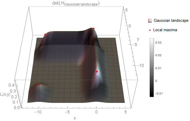
We want to compare these first moment updates with classical gradient descent. The following figure shows the example function and allows you to play around with a trajectory which starts near the summit of the hill.
Figure 1: Error function3 with a small local minimum before a larger minimum together with a trajectory which starts at the top hill. The trajectory is created via \eqref{eq:AdamOptimizer_AdamFirstMoment}. If you set \(\beta_1 = 0\), then the path corresponds to classical gradient descent. For \(\beta_1 > 0\), the first-order moments are included in the update process and for \(\beta_1 \geq 0.91\), the trajectory reaches the lower minimum. The learning rate is set to \(\eta = 20\) (relatively high since the error function has a low scaling).
Directly after the first descent is a small local minimum and we see that classical gradient descent (\(\beta_1 = 0\)) gets stuck here. However, with first-order moments (e.g. \(\beta_1 = 0.95\)), we leverage the fact that the moving average decreases not fast enough so that we can still roll over this small hole and make it down to the valley.4
We can see from the error landscape that the first gradient component has the major impact on the updates as it is the direction of the steepest hill. It is insightful to visualize the first component \(m_1(t)\) of the first-order moments over iteration time \(t\):
Figure 2: First component \(m_1(t)\) of the first-order moments over iteration time \(t\). The values are calculated according to \eqref{eq:AdamOptimizer_AdamFirstMoment} and use the same starting point as the trajectory in the previous figure. 150 iterations and a global learning rate of \(\eta=20\) were used. The \(\beta_1 = 0\) curve corresponds to classical gradient descent and the \(\beta_1 = 0.95\) curve to an update scheme which employs first-order moments.
With classical gradient descent (\(\beta_1 = 0\)), we move fast down the hill but then get stuck in the first local minimum. As only local gradient information is used in the update process, the chances of escaping the hole are very low.
In contrast, when using first-order moments, we increase slower in speed as only a fraction of the large first gradients is used. However, \(m_1(t)\) also decreases slower when reaching the first hole. In this case, the behaviour of the moving average helps to step over the short increase and to move further down the valley.
Building momentum and accelerating when we move in the same direction in subsequent iterations is the main concept and advantage of momentum optimization. However, as we already saw in the toy example used in the momentum optimizer article, large momentum vectors may be problematic as they can overstep local minima and lead to oscillations. What is more, as stressed in the argument above, it is not entirely clear if momentum optimization works well together with adaptive learning rates. Hence, it might be reasonable that the momentum optimizer is not used directly in Adam.
The final change in the Adam optimizer compared to its predecessors is the bias correction terms where we divide both moment vectors by either \((1-\beta_1^t)\) or \((1-\beta_2^t)\). This is because the moment vectors are initialized to zero so that the moving averages are, especially in the beginning, biased towards the origin. The factors are a countermeasure to correct this bias.
Practically speaking, these terms boost both vectors in the beginning since they are divided by a number usually \(< 1\). This can speed-up convergence when the true moving averages are not located at the origin but are larger instead. As the factors have the iteration number \(t\) in the exponent of the hyperparameters, the terms approach 1 over time and hence become less influential.
We now consider, once again, a one-dimensional example and define measures to compare the update vectors of the second iteration using either classical gradient descent or the Adam optimizer. To visualize the effect of the bias-correction terms, we repeat the process in which we leave these terms out.
Denoting the gradients of the first two iterations as \(g_t = \nabla E\left( w(t-1) \right)\), we build the moment estimates
To make the effect of the bias correction terms more evident, we moved them out of the compound fraction and used them as prefactor. We define a similar measure without these terms
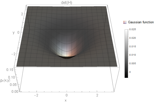
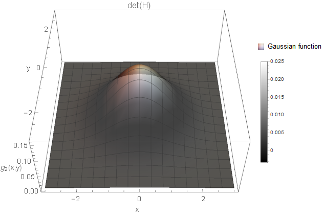
The following figure compares the two measures by interpreting the gradients of the first two iterations as variables.
Figure 3: Effect of the bias correction terms in the Adam optimizer. The left plot shows the measure \(C_A(g_1,g_2)\) (\eqref{eq:AdamOptimizer_AdamMeasureCorrection}) and the right \(\tilde{C}_A(g_1,g_2)\) (\eqref{eq:AdamOptimizer_AdamMeasureNoCorrection}). In the former measure, bias correction terms are used and in the latter not. Both measures compare the updates of Adam optimizer with the ones of classical gradient descent. The learning rate is set to \(\eta = 1\), the smoothing term to \(\varepsilon = 10^{-8}\) and the exponentially decaying rates to \(\beta_1 = 0.9\) and \(\beta_2 = 0.999\).
With correction terms (left image), we can observe that small gradients get amplified and larger ones attenuated. This is an inheritance from the adaptive learning scheme. Back then, however, this behaviour was more centred around the origin whereas here smaller gradients get amplified less and more independently of \(g_1\). This is likely an effect of the \(m(2)\) term which uses only a small fraction (10 % in this case) of the first gradient \(g_1\) leading to a smaller numerator.
When we compare this result with the one without any bias corrections (right image), we see a much brighter picture. That is, the area of amplification of small and attenuation of large gradients is stronger. This is not surprising, as the prefactor
is smaller than 1 and hence leads to an overall decrease (the term \((1-\beta_2^2) \cdot \varepsilon \) is too small to have a visible effect). Therefore, the bias correction terms ensure that the update vectors behave also more moderately at the beginning of the learning process.
Like in previous articles, we now also want to compare different trajectories when using the Adam optimizer. For this, we can use the following widget which implements the Adam optimizer.
Figure 4: Error surface of the function together with a trajectory of weight updates (top) and the error course corresponding to the weight updates (bottom). The trajectory is created according to the Adam optimizer with the smoothing term being set to \(\varepsilon = 10^{-8}\). You can specify your own error function5 and adjust the parameters via the slider. Click on the error surface to select a different starting point. The colour of the trajectory ranges from a dark to a bright blue with increasing iterations. You can make the course of the momentum components \(\fvec{m} = (m_1, m_2)\) and the scaling components \(\fvec{s} = (s_1, s_2)\) visible via the legend.
Basically, the parameters behave like expected: larger values for \(\beta_1\) make the accumulated gradients decrease slower so that we first overshoot the minimum. \(\beta_2\) controls again the preference of direction (\(\beta_2\) small) vs. magnitude (\(\beta_2\) large).
It is to note that even though the Adam optimizer is much more advanced than classical gradient descent, this does not mean that it is immune against extreme settings. It is still possible that weird effects happen like oscillations or that the overshooting mechanism discards good minima (example settings). Hence, it may still be worth it to search for good values for the hyperparameters.
We finished with the main concepts of the Adam optimizer. It is a popular optimization technique and its default settings are often a good starting point. Personally, I have had good experience with this optimizer and would definitely use it again. However, depending on the problem, it might not be the best choice or requires tuning of the hyperparameters. For this, it is good to know what they do and also how the other optimization techniques work.
List of attached files:
AdamOptimizer.nb [PDF] (Mathematica notebook with some basic computations and visualizations used to write this article)
This is the second part of a series consisting of three articles with the goal to introduce some general concepts and concrete algorithms in the field of neural network optimizers. As a reminder, here is the table of contents:
In the optimization techniques discussed previously (classical gradient descent and momentum optimizer), we used a global learning rate \(\eta\) for every weight in the model. However, this might not be a suitable setting as some neurons can benefit from a higher and others from a lower learning rate. What is more, per-neuron learning rates can help the weights move more in lockstep in the error landscape. This can be beneficial in approaching an optimum.
In a neural network with maybe thousands and thousands of parameters, we certainly do not want to adjust them all by hand. Hence, an automatic solution is required. There are multiple approaches to tackle this problem1. Here, we introduce the concept of adaptive learning rates which apply a different scaling to each gradient according to information from previous gradients essentially changing the learning rate.
The optimization technique we describe here follows the RMSProp algorithm introduced by Tieleman and Hinton in 2012. This is again an advancement of the AdaGrad method which was proposed in 2011 by Duchi, Hazan and Singer. We stick to the advanced version and refer to it as the adaptive learning scheme.
There is a second family of problems with relevance to this context. There are two extreme cases of gradient descent which can become problematic. On the one hand, there is the problem of plateaus in the error landscape. There, the gradient is very low and hence learning happens only very slowly. It would be nice to escape from these plateaus faster. Related to this problem are vanishing gradients, which can occur especially in deep neural networks, originating from the multiplication of small numbers (e.g. due to a plateau) and leading to even smaller numbers. If the gradients were larger, we could alleviate these problems.
On the other hand, gradients can also get very large, e.g. when moving across a steep hill in the error landscape. There, at least some components of the gradients are very large. If the steps are too big, we may overstep local minima hampering the goal of finding a good solution. Related to this are exploding gradients where gradients can grow uncontrollably fast due to the multiplication of large numbers. Even though less likely than vanishing gradients, they can still be problematic. If the gradients were smaller, we could alleviate these problems as well.
Generally speaking, problems can occur when gradients become either too large or too small. One goal is to keep the gradients in “reasonable ranges”. That is, amplify very small and attenuate very large gradients so that the problems discussed are less likely. Using an update scheme with adaptive learning rates can help.
An additional advantage of adaptive learning rates is that the global learning rate \(\eta\) needs much less tuning because each weight adapts its learning speed on its own. This leaves \(\eta\) being more of a general indicator than a critical design choice. To put it differently, the damage which can be caused by \(\eta\), e.g. by setting it way too high, is far smaller as each weight also applies its own scaling.
We are starting by defining the update rules for the adaptive learning scheme. We then look at a small numerical example, play around with trajectories in the error landscape and discuss some general concepts. Last but not least, there is also a new hyperparameter on which we want to elaborate. We skip speed comparisons as this would require a more realistic error function which can leverage some of the advantages of the procedure (e.g. faster escape from plateaus).
The basic extension of the adaptive learning scheme, compared to classical gradient descent, is the introduction of scaling factors \(\fvec{s}\) for each weight.
Additionally to the variables used in classical gradient descent, let \(\fvec{s} = (s_1, s_2, \ldots, s_n) \in \mathbb{R}^n\) be a vector with scaling factors for each weight in \(\fvec{w}\) initialized to zero, i.e. \(\fvec{s}(0) = \fvec{0}\), \(\beta \in [0;1]\) the decaying parameter and \(\varepsilon \in \mathbb{R}_{>0}\) a smoothing term. Then, the update rules
define the adaptive learning scheme and find a path from the initial position \(\fvec{w}(0)\) to a local minimum of the error function \(E\left(\fvec{w}\right)\). The symbol \(\odot\) denotes the point-wise multiplication and \(\oslash\) the point-wise division between vectors.
The scaling factors \(\fvec{s}\) accumulate information about all previous gradients in their squared form so that only the magnitude and not the sign of the gradient is changed. The squaring has the advantage (e.g. compared to the absolute value) that small gradients get even smaller and large gradients even larger so that their contribution in the scaling factors \(\fvec{s}\) is boosted. This intensifies the effects of the adaptive learning rates which we discuss below.
The hyperparameter \(\beta\) controls the influence of the previous scales \(\fvec{s}(t-1)\) compared to the influence of the new gradient \(\nabla E \left( \fvec{w}(t-1) \right)\). We are going to take a look at this one a bit later.
In each step, the weights now move in the direction of the update vector
which scales the gradient according to the square root of \(\fvec{s}\) effectively reverting the previous squaring step. Additionally, a small smoothing term \(\varepsilon\) to avoid division by zero is used. It is usually set to a very small number, e.g. \(\varepsilon = 10^{-8}\).
With the mathematical toolbox set up, we are ready to start with a small numerical example where we compare classical gradient descent with adaptive learning rates. We are using the same error function as before, i.e.
We do not change the parameters for classical gradient descent so the results \(\fvec{w}_c(1) = (-14.91, 19.6)\) and \(\fvec{w}_c(2) \approx (-14.82, 19.21)\) remain valid.
We set the decaying parameter to \(\beta = 0.9\) and the smoothing term to \(\varepsilon = 10^{-8}\). This leaves only the global learning rate to clarify. As we do not change the classical gradient descent approach, this leaves \(\eta_c = 0.001\). This is not an appropriate rate for the adaptive scheme, however. Due to the attenuation of higher gradients, this value is way too low so that we would not make much progress. We increase it therefore to2\(\eta_a = 0.05\). This would make speed comparisons more difficult but since we are not intending to do them, this is of no concern.
It is not a coincidence that the fractional part \(.84\) is the same for both vector components of \(\fvec{w}_a(1)\). This is because we initialized the scaling factors to \(\fvec{s}(0) = \fvec{0}\) so that only the squared gradient times \(1-\beta\) remain. In the weight update step, the gradient cancels nearly out due to the square root. In the end, both weight components change roughly by the same value (\(\approx +0.16\) for the first and \(\approx -0.16\) for the second component). Only the direction, indicated by the sign of the gradient, is different (we move to the right for \(w_1\) and to the left for \(w_2\)). We take up this point again later.
The new weight position \(\fvec{w}_a(1)\) is the basis to evaluate the next gradient
This situation is also visualized in the following figure.
Figure 1: Comparison of classical gradient descent (blue) with the adaptive learning scheme (orange). The two weight updates of the numerical example are shown. The weight vectors \(\fvec{w}\), the gradients \(\nabla E\) (used directly in classical gradient descent) in blue and the update vectors \(\fvec{v}(t)\) (\eqref{eq:Optimizer_AdaptiveUpdateVector}) of the adaptive learning rate scheme in orange are shown. Hover over the points to get more information.
The picture here is quite different from the momentum optimizer example. The difference is not in how far the vectors move (this would be hard to compare anyway due to the different learning rates) but rather how they move. With adaptive learning rates, we move more to the right and less to the bottom than with classical gradient descent.
Similar to what we did in momentum optimization, we want to know how the sequence from the example proceeds further. For this, you can play around in the following animation. It is the same as in the previous article except that the update sequence now uses adaptive learning rates.
Figure 2: Error surface of the function together with a trajectory of weight updates (top) and the error course corresponding to the weight updates (bottom). The trajectory is created according to the adaptive learning scheme with the smoothing term being set to \(\varepsilon = 10^{-8}\). You can specify your own error function3 and adjust the parameters via the slider. Click on the error surface to select a different starting point. The colour of the trajectory ranges from a dark to a bright blue with increasing iterations. You can make the course of the scaling components \(\fvec{s} = (s_1, s_2)\) visible via the legend.
We can see that with adaptive learning rates the trajectory is very different from classical gradient descent. Instead of moving down the steepest hill and then walking along the horizontal direction of the valley, the adaptive route points more directly towards the optimum. In this case, this results in a shorter path.
This is an effect of the general principle that the adaptive scheme tends to focus more on the direction than on the magnitude of the gradient. In momentum optimization, on the other side, we mainly focused on improving the magnitude. We even accepted small divergences from the optimal path for larger step sizes (cf. the oscillations of an \(\alpha = 0.9\) path). The opposite is the case with adaptive learning rates. Here, we focus more on the direction of the gradient vector instead of the magnitude.
The reason behind this lies in the scaling by the \(\fvec{s}\) vector. On the one hand, when the previous gradients were high so that the scaling factor is \(\sqrt{\fvec{s} + \varepsilon} > 1\), then the update step is reduced. On the other hand, with small previous gradients, the scaling factor is \(\sqrt{\fvec{s} + \varepsilon} < 1\) which increases the update step. This happens for each vector component individually.
The scaling has the effect that the magnitude of the gradient becomes less important as the update vectors \(\fvec{v}(t)\) are more forced to stay in “reasonable ranges”. This design was chosen with the intent to overcome the aforementioned problems of extremely small or large gradients. However, it is to note that the sign of the gradient is unaffected by this scaling which ensures that the update vector \(\fvec{v}(t)\) points always in the same direction as the gradient \(\nabla E(t)\).
In our example, this means that the vertical vector component decreases more since the gradients are higher in this direction (this is the direction with the steepest decline). As a result, the update vectors \(\fvec{v}\) point more to the right than with classical gradient descent. In the case of elongated error functions, this helps to point more directly at the optimum.
When we compare a \(\beta = 0\) with a \(\beta = 0.9\) trajectory, we see that the former is shaped more angularly and the latter is smoother. This is the case because the \(\beta = 0.9\) path does involve, at least to some extent, the magnitude of the gradients in the update decisions so that effectively a broader range of orientations is incorporated in the path. With \(\beta = 0\), however, we mainly restrict the path to the eight cardinal directions, e.g. in this case first to the south-east (\(\fvec{v} \approx (1, -1)\)) and then to the south (\(\fvec{v} \approx (0, -1)\)).
We discussed that with adaptive learning rates the focus is more on the direction than on the magnitude of the gradients. A valid question may be whether we have control over this focus. It turns out that we can use the hyperparameter \(\beta\) for this purpose and this is what we want to discuss now.
Let us begin with the extreme cases. When we set \(\beta = 0\), we do not use information from previous gradients and use only the current gradient instead. This is essentially what happened in the first update step of the numerical example (\eqref{eq:AdaptiveLearning_AdaptiveStep1}) where both vector components were updated by roughly the same value4. As we saw, this cancelled the magnitude of the gradient nearly completely out giving a strong importance to the sign. This is a way of expressing an exclusive focus on the direction.5
Setting \(\beta = 1\) does not use the current gradient in the scaling vector \(\fvec{s}\). Instead, only the initial value \(\fvec{s}(0)\) is used. In the case of zero-initialization, this leaves \(\sqrt{\varepsilon}\), i.e. a very small number, in the denominator so that an increase of the magnitude \( \left| \nabla E \left( \fvec{w}_a(1) \right) \right| \) is likely. In a way, this is an extreme focus on the magnitude. However, it is doubtful that this is a useful case as it contradicts the goal of keeping the update vectors in “reasonable ranges”.
For values in-between, i.e. \(\beta \in \; ]0;1[\), we have the choice of focusing more on the direction (smaller values of \(\beta\)) or more on the magnitude (larger values of \(\beta\)). For the latter, it is to note that the upper limit is not the original magnitude. Rather, it is possible that the magnitude even amplifies, as in the case of the extreme value \(\beta = 1\).
We now want to analyse how the update vectors \(\fvec{v}\) of the adaptive learning scheme are different from the gradients \(\nabla E\) used directly in classical gradient descent. For this, we use a one-dimensional example, consider two update iterations and interpret the gradients \(g_t = \nabla E \left( w(t-1) \right)\) as variables. We can then set up the scaling values
The question now is in which way the update value \(v(2)\) is different from the gradient \(g_2\), i.e. how we move differently with adaptive learning rates than without. More precisely, we want to know if the original gradient is amplified or attenuated. The idea is to measure this as a simple difference between the two update schemes:
The measure \(C_a(g_1, g_2)\) informs us about whether we move further in the adaptive learning scheme compared to classical gradient descent. This is, again, a sign-dependent decision as moving further means more to the right of \(g_2\) when \(g_2\) is already positive and more to the left of \(g_2\) when \(g_2\) is already negative.
When we interpret the sign and the magnitude of \(C_a(g_1, g_2)\), we can distinguish between the following cases:
For \(C_a(g_1, g_2) > 0\), the magnitude of the gradient \(|g_2|\) is amplified by \(\left| C_a(g_1, g_2) \right|\). The update step is larger with adaptive learning rates than without.
For \(C_a(g_1, g_2) < 0\), the magnitude of the gradient \(|g_2|\) is attenuated by \(\left| C_a(g_1, g_2) \right|\). The update step is smaller with adaptive learning rates than without.
For \(C_a(g_1, g_2) = 0\), the magnitude of the gradient \(|g_2|\) remains unchanged. The update step is the same with both approaches.
The following figure visualizes \eqref{eq:AdaptiveLearning_AdaptiveDifference} for different values of the hyperparameter \(\beta\).
Figure 3: Amplification or attenuation of the gradient with adaptive learning rates. The figures show the measure \(C_a(g_1, g_2)\) of \eqref{eq:AdaptiveLearning_AdaptiveDifference} which compares the update value \(v(2)\) of the adaptive learning scheme with the gradient \(g_2\) used directly in classical gradient descent. The colour shows whether the update with adaptive learning is greater than without (\(|v(2)| > |g_2|\), red regions) or less than without (\(|v(2)| < |g_2|\), blue regions). The smoothing term is set to \(\varepsilon = 10^{-8}\) and the global learning rate to \(\eta = 1\).
The red regions show where the gradient \(g_2\) is enlarged (first case). We see that this happens especially in areas where the value of both gradients is low. This is what helps us leaving a plateau of the error landscape escaping more quickly also alleviating the problem of vanishing gradients.
In the blue regions, the gradient \(g_2\) gets smaller. This corresponds to the second case. We see that these regions are visible strongest at the borders. That is, when either \(g_1\) or \(g_2\) are high (or both). This makes sure that the gradients do not become too large so that steep hills in the error landscape pose a risk of overstepping local minima. Smaller gradients also alleviate the problem of exploding gradients.
When we compare the result of different \(\beta\)-values, we can see how the focus changes from the direction to the magnitude of the gradients. The extreme value \(\beta = 0\) reveals a nearly linear relationship between \(v(2)\) and \(g_2\) as the magnitude is almost completely neglected setting the update essentially to \(\left| v(2) \right| \approx 1\).
This was also the story about adaptive learning rates. The global learning rate \(\eta\) does not have the power to suit the needs for every weight. Hence, using an individual learning rate (via the scaling vector \(\fvec{s}\)) per weight is a great and powerful idea which is also an important aspect of the Adam optimizer (covered in the next article). It is also nice that the scaling factors are calculated automatically. But, to be fair, we also do not have much of a choice since there is no practical way we could manually adjust the learning rates for each weight in a larger network.
Another advantage is that the global learning rate \(\eta\) becomes a less critical hyperparameter to adjust. Even though it still has an influence (otherwise, we could remove it), the effects are less drastic. This also means that it can cause less damage when it is set incorrectly.
A neural network is a model with a lot of parameters which are used to derive an output based on an input. In the learning process, we show the network a series of example inputs with an associated output so that it can adapt its parameters (weights) according to a defined error function. Since these error functions are too complex, we cannot simply determine an explicit formula for the optimal parameters. The usual approach to tackle this problem is to start with a random initialization of the weights and use gradient descent to iteratively find a local minimum in the error landscape. That is, we adapt the weights over multiple iterations according to the gradients until the value of the error function is sufficiently low.
However, using this approach without modifications (classical gradient descent) has some disadvantages as it can be slow, may end up in a suboptimal local minimum and requires a careful choice of the learning rate. Hence, multiple approaches have been developed over the years to improve classical gradient descent and address a few of the problems.
This is the first part of a series consisting of three articles with the goal to introduce some general concepts and concrete algorithms in the field of neural network optimizers. We start in in this article with the momentum optimizer which tries to improve convergence by speeding up when we keep moving in the same direction. The second part introduces the concept of individual learning rates for each weight in the form of an adaptive learning scheme which scales according to the accumulation of past gradients. Finally, the third part introduces the Adam optimizer which re-uses some of the ideas discussed in the first two parts and also tries to target better local minima. In summary:
In classical gradient descent, we perform each update step solely on the basis of the current gradient. In particular, no information about the previous gradients is included in the update step. However, this might not be very beneficial as the previous gradients can provide us with information to speed up convergence. This is where the momentum optimizer comes into play.1.
The general idea is to speed up learning when we move in the same direction over multiple iterations and we slow down when the direction changes. With “direction” we mean the sign of the gradient components as we update each weight individually. For example, if we had moved to the right in the first two iterations (positive gradient components), we could assume that our optimum is somewhere at the right and move even a bit further in this direction. Of course, this decision is only possible when we still have the information about the gradient of the first iteration.
There is an analogy which is often used: imagine we place a ball at a hill and it rolls down into a valley. We use gradient descent to update the position of the ball based on the current slopes. If we use classical gradient descent, it is like placing the ball each time on the new position completely independent of the previous trajectory. With momentum optimization, however, the ball accelerates in speed as it builds momentum2. This allows the ball to reach the valley much faster than with classical gradient descent.
There is one problem with the current approach, though: if we accelerated uncontrolledly as long as we move in the same direction, we might end up with huge update steps predestined to overshoot local minima. Hence, we need some kind of friction mechanism to act as a counterforce to slow down the ball again.
In the following, we introduce the concepts behind momentum optimization. We begin with the mathematical formulation where we also compare it with classical gradient descent. We then apply the formulas on a small numerical example to understand their basic functionality and look at different trajectories. Next, we analyse the speed improvements of momentum optimization from an exemplary and theoretical point of view. Lastly, we discuss the two basic concepts in momentum optimization, namely acceleration and deceleration, in more detail.
The basic algorithm to iteratively find a minimum of a function is (classical) gradient descent. It uses, as the name suggests, the gradients \(\nabla E\) of the error function \(E\left(\fvec{w}\right)\) as the main ingredient.
Let \(\fvec{w} = (w_1, w_2, \ldots, w_n) \in \mathbb{R}^n\) be a vector of weights (e.g. of a neural network) initialized randomly at \(\fvec{w}(0)\), \(\eta \in \mathbb{R}^+\) a global learning rate and \(t \in \mathbb{N}^+\) the iteration number. Then, classical gradient descent uses the update rule
to find a path from the initial position \(\fvec{w}(0)\) to a local minimum of the error function \(E\left(\fvec{w}\right)\) based on the gradients \(\nabla E\).
That is, we move in each iteration in the direction of the current gradient vector (the gradient is subtracted since we want to reach a minimum and not a maximum of \(E(\fvec{w})\) in gradient descent). In momentum optimization, we move in the direction of the momentum vector \(\fvec{m}\) instead.
Additionally to the variables used in classical gradient descent, let \(\fvec{m} = (m_1, m_2, \ldots, m_n) \in \mathbb{R}^n\) be the momentum vector of the same length as the weights \(\fvec{w}\) which is initialized to zero, i.e. \(\fvec{m}(0) = \fvec{0}\), and \(\alpha \in [0;1]\) the momentum parameter (friction parameter). Then, the momentum optimizer defines the update rules
to find a path from the initial position \(\fvec{w}(0)\) to a local minimum of the error function \(E\left(\fvec{w}\right)\).
These equations summarize the former ideas: we keep track of previous gradients by adding them to the momentum vector, we subtract the momentum vector \(\fvec{m}\) which includes information about the complete previous trajectory and we have a friction mechanism in terms of the momentum parameter \(\alpha\).
If we set \(\alpha = 0\), we do not consider previous gradients and end up with classical gradient descent, i.e. \eqref{eq:MomentumOptimizer_ClassicalGradientDescent} and \eqref{eq:MomentumOptimizer_Momentum} produce the same sequence of weights. In the other extreme, \(\alpha = 1\), we have no friction at all and accumulate every previous gradient. This is not really a useful setting as the updates tend to get way too large so that we almost certainly overshoot every local minimum. For values in-between, i.e. \(\alpha \in \; ]0;1[\), we can control the amount of friction we want to have with lower values of \(\alpha\) meaning a higher amount of friction as more of the previous gradients are discarded. We are comparing different values for this hyperparameter3 later.
First, let us look at a numerical example which compares classical gradient descent with momentum optimization. For this, suppose that we have two weights \(w_1\) and \(w_2\) used in the (fictional) error function
We are starting in our error landscape at the position \(\fvec{w}(0) = (-15,20)\), using a learning rate of \(\eta = 0.001\) and want to apply two updates to the weights \(\fvec{w}\). We first need to calculate the gradients of our error function
We now repeat the same process but with momentum optimization enabled and the momentum parameter set to \(\alpha = 0.9\). Since the momentum vector is initialized to \( \fvec{m}(0) = \fvec{0} \), the first update is the same as before
In the second update, however, the momentum optimizer leverages the fact that we move again in the same direction (\(w_1\) to the right and \(w_2\) to the left) and accelerates (the gradient is the same as before, i.e. \(\nabla E \left( \fvec{w}_m(1) \right) = \nabla E \left( \fvec{w}_c(1) \right)\))
This situation is also visualized in the following figure:
Figure 1: Comparison of gradient descent with (orange) and without (blue) momentum optimization after the second weights update of the numerical example. The weight vectors \(\fvec{w}\), the gradients \(\nabla E\) and the momentum vectors \(\fvec{m}\) are shown. Hover over the points to get more information. It is also possible to disable a line by clicking on the legend.
We can see that the position with momentum \(\fvec{w}_m(2)\) is a fair way ahead of the position \(\fvec{w}_c(2)\) reached via classical gradient descent. That is, the first weight moved more to the right (\(w_{1,m}(2) > w_{1,c}(2)\)) and the second weight more to the left (\(w_{2,m}(2) < w_{2,c}(2)\)).
So, how do the two approaches proceed further on their way to the minimum? To answer this question, you can play around in the following animation. With the default error function and without considering extreme settings, all trajectories should find their way to the local (and in this case also global) minimum of \(\fvec{w}^* = (0, 0)\).
Figure 2: Error surface of the function together with a trajectory of weight updates (top) and the error course corresponding to the weight updates (bottom). The trajectory is created with the momentum optimizer and updated according to \eqref{eq:MomentumOptimizer_Momentum}. You can specify your own error function5 and adjust the parameters via the slider. If you set \(\alpha = 0\), then the path corresponds to classical gradient descent. Click on the error surface to select a different starting point. The colour of the trajectory ranges from a dark to a bright blue with increasing iterations. You can make the course of the momentum components \(\fvec{m} = (m_1, m_2)\) visible via the legend.
If we start with classical gradient descent (\(\alpha = 0\)) and then increase the momentum parameter \(\alpha\), we see how we reach closer to the minimum in the same number of iterations. However, setting the parameter too high can lead to negative effects. For example, the \(\alpha = 0.9\) path first moves in the wrong direction (down) before it turns back to the minimum. This is a consequence of too little friction. The accumulation from the first few gradients is still very high so that the step sizes are very large (enable the \(m_2\) trace to make this effect more prominent). It takes some iterations before the friction can do its job and decreases the accumulation so that the path can turn and move into the correct direction again. This happens once more when the path is already near the local minimum (zoom in to see this better).
Generally speaking, when we set the momentum parameter \(\alpha\) too high, it is likely to happen that the path oscillates around an optimum. It may overshoot the minimum several times before the accumulated values decreased enough.
Of course, instead of adjusting the momentum parameter \(\alpha\), we could also tune the learning rate \(\eta\). Increasing it can also help to reach the minimum faster and it can lead to similar oscillation problems6. However, \(\eta\) is a global setting and influences all step sizes independent of the current location in the error surface. The momentum parameter \(\alpha\), on the other hand, specifies how much we take from the currently accumulated momentum and this depends on all previous gradients. What is more, a good setting for the learning rate \(\eta\) helps also in momentum optimization.
It is to note that in neural networks, with usually many more parameters than just two, it is not easily possible to visualize the trajectory as it is done here. One has to trust other measures, like the value of the error function \(E(\fvec{w})\), instead.
The goal of momentum optimization is to converge faster to a local optimum and we can see that this is indeed the case when we keep track of the error course. To make this comparison even clearer, we are elaborating on this point a bit further in this section.
One note before we proceed, though: the results here serve only as a general hint and do not necessarily represent realistic speed improvements. That is because we use \eqref{eq:MomentumOptimizer_ExampleFunction} as error function which is only a toy example. Error surfaces from the real world are usually more complex so that optimizers may behave differently.
However, the nice thing about this error function is that it has only one minimum so that any reduction of the error value means that we come closer to the same optimum. This allows us to compare the value of the error function in each step \(t\). This is done in the following figure for three different trajectories with different values for the momentum parameter \(\alpha\). The lower the value on the \(y\)-axis, the closer is the path to the minimum and the earlier this happens, the better.
Figure 3: Comparison of the convergence speed of three trajectories using different values for the momentum parameter \(\alpha\) over the course of 700 iterations. The other parameters are set to the initial values of the previous figure. The \(y\)-axis is not shown in its full range to restrict the comparison to its relevant parts.
We can clearly see that with classical gradient descent (\(\alpha = 0\)) we reach the optimum slowest compared to the other curves. Using the momentum optimizer helps here in both cases with \(\alpha = 0.9\) being even a bit faster than \(\alpha = 0.6\). However, we also see the problems of the \(\alpha = 0.9\) curve which has a small bump at around \(t = 20\). This is when the corresponding trajectory moves too much to the south of the error function before turning to the optimum.
Regarding the speed improvements, there is also a theoretical argument we want to stress here. It concerns a possible theoretical speedup with momentum optimization. We use a one-dimensional example and assume that the gradient \(g\) stays constant during all iterations. We can then calculate the sequence of momentum updates
\begin{align*}
m(0) &= 0 \\
m(1) &= \alpha \cdot m(0) + g = g \\
m(2) &= \alpha \cdot m(1) + g = \alpha \cdot g + g \\
m(3) &= \alpha \cdot m(2) + g = \alpha \cdot (\alpha \cdot g + g) + g = \alpha^2 \cdot g + \alpha \cdot g + g \\
&\vdots \\
m(t) &= \sum_{i=0}^{t-1} \alpha^i \cdot g \Rightarrow \lim\limits_{t \rightarrow \infty} g \sum_{i=0}^{t-1} \alpha^i = g \frac{1}{1-\alpha}.
\end{align*}
In the last step, we assumed \(|\alpha| < 1\) and used the limit of the geometric series to simplify the formula.
As we can see, the influence of previous gradients decreases exponentially. In total, momentum optimization effectively pushes the gradient by a factor depending on the momentum parameter \(\alpha\). For example, if we use \(\alpha = 0.9\), we get a speedup of \(\xfrac{1}{0.1} = 10\) for the last update. That is, the weight updates are up to 10 times larger than without momentum optimization.
It is to note that this is only a theoretical perspective and the simplification of constant gradients is not very realistic. After all, we could just adapt the learning rate with increasing iterations to achieve a similar effect in this case. Still, it gives a general idea of the convergence improvements from momentum optimization and which role the hyperparameter \(\alpha\) plays.
So far, we focused mainly on the acceleration functionality of momentum optimization. As we saw, we accelerate when we move in the same direction as in the previous iteration7. That is, the magnitude of the momentum vector increases, i.e. \( \left\| \fvec{m}(t) \right\| > \left\| \fvec{m}(t-1) \right\| \). On the other hand, we decelerate when we change directions. In this case, the magnitude of the momentum vector decreases, i.e. \( \left\| \fvec{m}(t) \right\| < \left\| \fvec{m}(t-1) \right\| \). These are two fundamental cases in the momentum optimizer. We now want to discuss a bit deeper when and to which extent these cases apply.
To make things simpler, we use, again, one dimension so that only one weight and more importantly one gradient per iteration remains. We consider two iterations of the momentum update, interpret the gradients as variables \(g_1 = \nabla E \left( w(0) \right)\) for the first and \(g_2 = \nabla E \left( w(1) \right)\) for the second iteration:
The idea is to measure the acceleration and deceleration between the two momentum updates as a function of the gradients \(g_i\). We can do so by simply calculating the difference between \(m(1)\) and \(m(2)\) to see how much the momentum changes. However, since “the correct direction” (positive to the right, negative to the left) depends on the sign of the first gradient \(g_1\), we need to handle these cases separately:
For the measure \(C_m(g_1, g_2)\), we can interpret the sign and the magnitude leading to the following cases:
For \(C_m(g_1, g_2) > 0\), the gradient \(g_2\) points in the same direction as \(g_1\) and the magnitude \(\left| m \right| \) increases by \( \left|C_m(g_1, g_2)\right| \).
For \(C_m(g_1, g_2) < 0\), the gradient \(g_2\) points in the opposite direction as \(g_1\) and the magnitude \(\left| m \right| \) decreases by \( \left|C_m(g_1, g_2)\right| \).
For \(C_m(g_1, g_2) = 0\), the magnitude \(\left| m \right| \) remains unchanged. This is not really an interesting case and only listed for the sake of completeness.
Note that the reverse of the above statements is not true in general. For example, if the gradient \(g_2\) points in the same direction as \(g_1\), it does not necessarily mean that the magnitude of the momentum increases. Let \(g_1 = 2, g_2 = 1\) and \(\alpha = 0.4\) to make this point clear:
Both gradients point in the same direction but the momentum still changes by \(m(2) - m(1) = -0.2\), i.e. it gets smaller. This is due to the friction parameter \(\alpha\) and the second gradient being too small to account for the friction loss \(0.6 \cdot 2 = 1.2\).
The following figure visualizes \eqref{eq:MomentumOptimizer_Cases} graphically. The red regions correspond to the first case and the blue regions to the second case. Additionally, we see by the intensity of the colour how much the momentum changes. We are building momentum in the bottom-left and top-right quarters, i.e. when the gradients share the same sign and the second gradient \(g_2\) can account for the friction loss.
Figure 4: Acceleration and deceleration between two momentum updates as a function of the gradients. The colour indicates the value of the function \(C_m(g_1, g_2)\) of \eqref{eq:MomentumOptimizer_Cases} which uses the momentum values \(m(1)\) and \(m(2)\) from the first two iterations (cf. \eqref{eq:MomentumOptimizer_CasesUpdates}). These, in turn, depend on the gradients \(g_1\) and \(g_2\). Essentially, the colour shows whether the magnitude \(\left| m \right| \) of the momentum increases (red regions) or decreases (blue regions). Note that the contour lines are degenerated in the \(g_1 = 0\) line since \eqref{eq:MomentumOptimizer_Cases} is not a continuous function. However, this is not relevant for our discussion.
The friction parameter \(\alpha\) influences the slope of the contour lines. It is highest for \(\alpha = 0\) where the previous gradient is ignored completely and the momentum term only increases when the new gradient is larger, i.e. \(g_2 > g_1\). This is not surprising as this case reduces to classical gradient descent where we do not have a momentum term. The slope is lowest (more precisely: zero) for \(\alpha = 1\). This is the case where we do not have any friction at all and sum up the full magnitudes of all previous gradients. Hence, when the second gradient has e.g. a value of \(g_2 = 1\), the momentum term increases by this value: \(m(2) - m(1) = 1\).
This was the story about momentum optimization. It introduces an important idea to speed up convergence in neural network optimization namely that we can be smarter when we keep moving in the same direction over iteration time. However, it should not be used without caution since the friction parameter \(\alpha\) highly influences our success. Setting it too low and we may learn slower than we could. Setting it too high and we may lose control over our trajectory in the error landscape. This is especially hard to catch for higher-dimensional error functions (usually the case in neural networks).
Even though the concept of momentum optimization has its right to exist, I have to admit that I can't remember ever using it on its own. There are usually enough (critical) hyperparameters in a network so that adjusting the friction parameter \(\alpha\) can be a bit scary. What is more, other optimization techniques have been developed which work reasonably well and have less critical hyperparameters.
A popular example is the Adam optimizer which reuses the idea of momentum even though in a different form and with different effects. We are also covering the Adam optimizer in this series about neural network optimization (third part). But before we are taking a look at this technique, we should first learn about a new concept: adaptive learning rates. This is also very important for the Adam optimizer.
List of attached files:
MomentumOptimizer.nb [PDF] (Mathematica notebook with some basic computations and visualizations used to write this article)
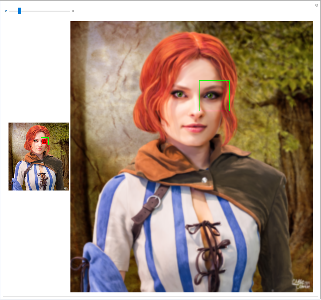
If you place images to a layout with a maximal width (like this webpage here), you may encounter the problem that you have images which are too large to display. Hence, the image is only shown in a lower resolution. But when we want the user to still be able to view the image in its full glory, we need an additional way of interaction. One could be to provide a link to the image in its full size but then the user has to leave the current page which breaks the attentional flow. A lightbox is a very common and nice way to overcome this issue which allows viewing images in higher resolutions without leaving the current site. The image is shown enlarged on the same page as before and the rest of the site is hidden in the background (but still visible) as seen in the following example.
Figure 1: Example image to show the lightbox (showing a dolphin).
In an abstract way, a lightbox has to handle two different states: the normal mode where the image is shown as usual on the site and the lightbox mode where the image is shown enlarged. Somehow the user must be able to switch between these states, e.g. by clicking on the enlarged image (or whatever you prefer).
Technically, there are different ways to realize lightboxes. A common approach is to use a JavaScript library. These have the advantage of abstracting most of the details for you but also requires that the user has JavaScript enabled and add additional bloat to the webpage since the JS code must be loaded as well. There are approaches, though, to realize lightboxes with pure HTML and CSS. One way is to use the :target pseudo-class selector (example) which works by using page anchors (e.g. #linkToSectionOfThisSite) to distinguish between the two states. However, this has the disadvantage of altering the user's browsing history, i.e. the back and forward navigation. If a user opened and closed a lightbox realized in this way, pressing the back button would result in showing the enlarged image again. Since this is not a user-friendly behaviour, in my opinion, I searched for a different solution which I am presenting in this article.
The idea is to use a hidden input element to handle the states and a corresponding label element which wraps the image and links it with the input tag. In HTML, this could be realized as
<!-- The input element is hidden and is only responsible for handling the state -->
<input id="lightbox:CSSLightbox_ExampleImage" class="lightbox" type="checkbox">
    <!-- The label connects the child image with the input element so that a click on the image corresponds to an event to the input element -->
<label for="lightbox:CSSLightbox_ExampleImage" title="Click to close">
  <!-- Image which is selectable by the user (in the article to enlarge and in the lightbox to close) -->
  <img src="/content-blog/Informatics/Web/CSSLightbox_ExampleImage.jpg" title="Click to show the image enlarged" alt="Example image for the lightbox (showing a dolphin)" width="300">
</label>
As you can see, a checkbox is re-used for our purpose and since the image is attached as a child to the label tag, every interaction with the image is an interaction with the label element which in turn triggers the state of the checkbox. You can't see that the input element is hidden since this is controlled via CSS:
.lightbox {
    /* Hide the input element */
    display: none;
    /* ... */
}
So, what is the intended change when the user clicks on the image? Obviously, the image should be displayed enlarged, but there is more: we want that the complete webpage is visible in the background – including the image itself (in its scaled-down size). The image inside the label tag is also used as lightbox image since only elements inside the label react on user interaction and we want that the user has also the ability to close the lightbox again. Hence, we need a duplicate of the image in the lightbox mode so that the original image is still shown in the background. This is realized via an additional image tag after the label element.
<!-- Background image shown in the article when the lightbox is active -->
<img src="/content-blog/Informatics/Web/CSSLightbox_ExampleImage.jpg" alt="Example image for the lightbox (showing a dolphin)" width="300">
Like before, the image is hidden by default and displayed again when the lightbox is active (via CSS, see below). As you may have noticed, there are also title attributes on the label and the img tags. They are used to guide the user with a default browser tooltip when hovering over the image in the normal mode (indicating that it can be enlarged) or when hovering over the label in the lightbox mode (indicating that it can be closed). Since the image is placed on top of the label, its title is normally shown. To make sure that the title of the label tag gets displayed in the lightbox mode, we have to disable the pointer events for the image1:
.lightbox:checked + label img {
    /* ... */
    /* Prevent that the title attribute of the image gets shown so that the title attribute of the label can be shown instead */
    pointer-events: none;
}
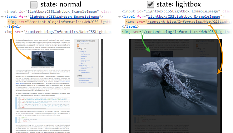
The following figure summarizes what we have so far and makes clear which image tag is responsible for what in which state.
Figure 2: The two states of the lightbox managed by a checkbox. Tags are greyed-out when they are hidden (via CSS, not shown here) in the respective state. The arrows indicate which img tag corresponds to which image on the webpage.
There are two open questions left: what layout changes do we need in the lightbox state and how do we distinguish between the two states in code under the constraint of not using JS? Both answers lie in the relevant CSS sections.
.lightbox:checked + label + img {
    /* Show the image in the text (both images should be visible) */
    display: block;
}
.lightbox:checked + label {
    /* Fade out the rest of the site so that the image appears in front */
    background: rgba(0,0,0,0.8);
    outline: none;

    /* Make sure that the lightbox is visible in front and fills the complete screen */
    position: fixed;
    z-index: 999;
    width: 100%;
    height: 100%;
    top: 0;
    left: 0;

    display: flex;              /* Allows easy alignment */
    justify-content: center;    /* Align vertically */
    align-items: center;        /* Align horizontally */

    /* ... */
}
.lightbox:checked + label > img {
    /* Show the image on a white background (better for transparent images) */
    background: white;

    /* Reset resolution to default */
    width: auto !important;
    height: auto !important;

    /* Don't fill the complete screen with the image, it should always be a bit from the site visible */
    max-width: 90%;
    max-height: 90%;

   /* Remove any outer filling which might lead to white borders (due to the background filling) */
    padding: 0;
    margin: 0;

    /* Prevent that the title attribute of the image gets shown so that the title attribute of the label can be shown instead */
    pointer-events: none;
}
The first block (lines 1–4) is responsible for showing the image in the article via the second img tag when the lightbox is active. In the second block (lines 5–23), we fade out the background, enlarge the label to the full size of the page and make sure that every element inside the label is displayed in the centre of the page. Note the use of flexbox which is a handy way of aligning elements of the page. In the third block (lines 24–42), we ensure that the image can be displayed in its full size but still leaving some margin to the borders (but this is only a matter of preferences).
Actually, the interesting part here is .lightbox:checked where the :checked pseudo-class is used to style the page differently depending on the state of the checkbox. The rule .lightbox:checked applies when the checkbox is active, i.e. via a click on the image in our case. But the rule does not stop there. E.g. in line 5 (.lightbox:checked + label) we actually select the first label via the adjacent sibling operator (+). This means, whenever the checkbox is in its checked state, we select the label which is placed after the input element and style this label (and not the input tag!) with the definitions of the lines 6–22.
This is quite interesting if you think about it. We relate the style of one element (label) with the state of another element (input). And the state control element does not even have to be visible. You can apply this technique in many scenarios. The only thing which you need to make sure is to place the two elements near to each other so that you can select them via the sibling combinators.
The following JSFiddle shows the complete code and lets you play around with it. Besides what I have shown so far, there is additional code in the CSS section covering some details I skipped (e.g. how to avoid some input selection glitches). I invite you to go through the comments if you are interested in these aspects.
Suppose you have some data and want to get a feeling about the underlying probability distribution which produced them. Unfortunately, you don't have any further information like the type of distribution (\(t\)-distribution, Poisson, etc.) or its parameters (mean, variance, etc.). Further, assuming a normal distribution does not seem to be the right thing. This situation is quite common in reality and the good news is that there are some helpful techniques. One is known as kernel density estimation (also known as Parzen window density estimation or Parzen-Rosenblatt window method). This article is dedicated to this technique and tries to convey the basics to understand it.
Parzen window is a so-called non-parametric estimation method since we don't even know the type of the underlying distribution. In contrast, when we estimate the PDF1 \(\hat{p}(x)\) in a parametric way, we know (or assume) the type of the PDF (e.g. a normal distribution) and only have to estimate the parameters of the assumed distribution. But, in our case, we really know nothing and hence need to find a different approach which is not based on finding the best-suited parameters. Further, we assume continuous data and hence work with densities instead of probabilities.2
Let's start by formulating what we have and what we want. Given is a set of \(N\) data points \(X = (x_1, x_2, \ldots, x_N)\) and our goal is to find a PDF which satisfies the following conditions:
The PDF should resemble the data. This means that the general structure of the data should still be visible. We don't require an exact mapping but groups in the dataset should also be noticeable as high-density values in the PDF.
We are interested in a smooth representation of the PDF. Naturally, \(X\) contains only a discrete list of points but the underlying distribution is most likely continuous. This should be covered by the PDF as well. More importantly, we want something better than a simple step function as offered by a histogram (even though histograms will be the starting point of our discussion). Hence, the PDF should approximate the distribution beyond the evidence from the data points.
The last point is already implied by the word PDF itself: we want the PDF to be valid. Mathematically, the most important properties which the estimation \(\hat{p}(x)\) must obey are \begin{equation}
\label{eq:ParzenWindow_PDFConstraints}
\int_{-\infty}^{\infty} \! \hat{p}(x) \, \mathrm{d}x = 1 \quad \text{and} \quad \hat{p}(x) \geq 0.
\end{equation} That is, the PDF should integrate up to 1 and every density value is non-negative.
The rest of this article is structured as follows: we are going to start with one-dimensional data and histograms. Even though this is not intended to be a full introduction to histograms, it is good starting point for our discussion. We are going to face the problems of classical histograms and the solution ends indeed in the Parzen window estimator. We are looking at the definition of the estimator and try to get some intuition about its components and parameters. It is also possible to reach the estimator from a different way, namely from the signal theory, by using convolution and we are going to take a look at this, too. In the last part, we are going to generalize the estimator to the multi-dimensional case and provide an example in 2D.
Histograms are a very easy way to get information about the distribution of the data. They show us how often certain data points occur in the whole dataset. A common example is an image histogram which shows the distribution of the intensity values in an image. In this case, we can simply count how often each of the 256 intensity values occurs and draw a line for each intensity value with the height corresponding to the number of times that intensity value is present in the image.
Another nice property of the histogram is that it can be scaled to be a valid discrete probability distribution itself (though, not a PDF yet3). This means we reduce the height of each line so that the total sum is 1. In the case of a image histogram, we can simply make the count a relative frequency by dividing by the total number of pixels and we end up with a valid distribution. To make this more concrete, let \(b_i\) denote the number of pixels with intensity \(i\) and \(N\) the total number of pixels in the image so that we can calculate the height of each line as
\(\hat{p}_i\) is then an estimate of the probability of the \(i\)-th intensity value (the relative frequency).
An image histogram is a very simple example because we have only a finite set of values to deal with. In other cases, the border values (e.g. 0 and 255 in the image example) are not so clear. What is more, the values might not even be discrete. If every value \(x \in \mathbb{R}\) is imaginable, the histogram is not very interesting since most of the values will probably occur only once. E.g. if we had the values 0.1, 0.11 and 0.112, they would end up as three lines in our histogram.
Obviously, we need something more sophisticated. Instead of counting the occurrences of each possible value, we collect them in so-called bins. Each bin has a certain width and we assign the values to whichever bin they are falling into. Instead of lines, we now draw bars and the height of each bar is proportional to the number of values which had been falling into the bin. For simplicity, we are assuming that each bin has the same width. Note, however, that this is not necessarily a requirement.
Let's redefine \(b_i\) to denote the number of values which are falling into the \(i\)-th bin. Can we still use \eqref{eq:ParzenWindow_ImageHistogram} to calculate the height of each bar when the requirement is now to obtain a valid PDF? No, we can't since the histogram estimate \(\hat{p}(x)\) would violate the first constraint of \eqref{eq:ParzenWindow_PDFConstraints}, i.e. the area of all bars does not integrate up to 1. This is due to the binning where we effectively expand each line horizontally to the bin width, i.e. we make it a rectangle. This influences the occupied area and we need some kind of compensation. But, the solution is very simple: we just scale the height by the bin width4 \(h > 0\)
\begin{equation}
\label{eq:ParzenWindow_Histogram}
\hat{p}(x) =
\begin{cases}
\frac{1}{h} \cdot \frac{b_i}{N} & \text{if \(x\) falls into the bin \(b_i\)} \\
0 & \text{else} \\
\end{cases}
\end{equation}
Let's create a small example which we can also use later when we dive into the Parzen window approach. We consider a short data set \(X\) consisting only of four points (or more precisely: values)
Suppose, we want to create a histogram with bins of width \(h=2\). The first question is: where do we start binning, i.e. what is the left coordinate of the first bin? 1? 0? -42? This is actually application-specific since sometimes we have a natural range where it could be valid to start e.g. with 0. In this case, however, there is no application context behind the data so let's just start at \(\min(X) = 1\). With this approach, we can cover the complete dataset with three bins (\(B_i\) denotes the range of the \(i\)-th bin)
The first two data points are falling into \(B_1\) and the other two in \(B_2\) and \(B_3\). We can calculate the heights of the bins according to \eqref{eq:ParzenWindow_Histogram} as
It is easy to see that this sums indeed up to \(2 \cdot 0.25 + 2 \cdot 2 \cdot 0.125 = 1\). The following figure shows a graphical representation of the histogram.
Figure 1: Histogram of the example data of \eqref{eq:ParzenWindow_ExampleData} normalized according to \eqref{eq:ParzenWindow_Histogram}. Besides the bins, the data points are also visualized as red points on the \(x\)-axis.
So, why do we need something else when we can already obtain a valid PDF via the histogram method? The problem is that histograms provide only a rough representation of the underlying distribution. And as you can see from the last example, \(\hat{p}(x)\) results only in a step function and usually we want something smoother. This is where the Parzen window estimator enters the field.
Our goal is to improve the histogram method by finding a function which is smoother but still a valid PDF. The general idea of the Parzen window estimator is to use multiple so-called kernel functions and place them at the positions of the data points. We are superposing all of these kernels and scale the result to our needs. The resulting function from this process is our PDF. We implement this idea by replacing the cardinality of the bins \(b_i\) in \eqref{eq:ParzenWindow_Histogram} with something more sophisticated (still for the one-dimensional case):
Definition 1: Kernel density estimation (Parzen window estimator) [1D]
Let \(X = (x_1, x_2, \ldots, x_N) \in \mathbb{R}^N\) be the column vector containing the data points \(x_i \in \mathbb{R}\). Then, we can use the Parzen window estimator
to retrieve a valid PDF which returns the probability density for an arbitrary \(x\) value. The kernels \(K(x)\) have to be valid PDFs and are parametrized by the side length \(h \in \mathbb{R}^+\).
To calculate the density for an arbitrary \(x\) value, we now need to iterate over the complete dataset and sum up the result of the evaluated kernel functions \(K(x)\). The nice thing is that \(\hat{p}(x)\) inherits the properties of the kernel functions. If \(K(x)\) is smooth, \(\hat{p}(x)\) tends to be smooth as well. That is, the kernel dictates how \(\hat{p}(x)\) behaves, how smooth it is and how each \(x_i\) contributes to any \(x\) which we plug into \(\hat{p}(x)\). A common choice is to use standard normal Gaussians which we are also going to use in the example later. What is more, it can be shown that if \(K(x)\) is a valid PDF, i.e. satisfying, among others, \eqref{eq:ParzenWindow_PDFConstraints}, \(\hat{p}(x)\) is a valid PDF as well!
Two operations are performed in the argument of the kernel function. The kernel is shifted to the position \(x_i\) and stretched horizontally by the side length \(h\) which determines the range of influence of the kernel. Similar to before, \(h\) specifies the number of points which contribute to the bins – only that the bins are now more complicated. We don't have a clear bin-structure anymore since the bins are now implemented by the kernel functions.
In the prefactor, the whole function is scaled by \(\xfrac{1}{h \cdot N}\). As before in \eqref{eq:ParzenWindow_Histogram}, this is necessary so that the area enclosed by \(\hat{p}(x)\) equals 1 (requirement for a valid PDF). This is also intuitively clear: as more points we have in our dataset, as more we sum up and to compensate for this we need to scale-down \(\hat{p}(x)\). Likewise, as larger the bin width \(h\), as wider our kernels get and as more points they consider. In the end, we have to compensate for this as well.
We now could directly start and use this approach to retrieve a smooth PDF. However, let's apply \eqref{eq:ParzenWindow_KernelDensity} first to a small example and this is easier when we stick to uniform kernels for a moment. This does not give us a smooth function, but hopefully some insights in the approach itself. The uniform kernels have a length of 1 and are centred around the origin
When we want to know how this kernel behaves, we must first talk about the kernel argument \(\xfrac{x_i - x}{h}\). How does the kernel change with this argument? As mentioned before, it stretches and shifts the kernel to the position of \(x_i\). To see this, let us replace \(x\) in \(0.5 \leq x \leq 0.5\) with our kernel argument:
\begin{align*}
&\phantom{\Leftrightarrow} -0.5 \leq \frac{x_i - x}{h} \leq 0.5 \\
&\Leftrightarrow -0.5 \cdot h \leq x_i - x \leq 0.5 \cdot h \\
&\Leftrightarrow -0.5 \cdot h \leq -(-x_i + x) \leq 0.5 \cdot h \\
&\Leftrightarrow 0.5 \cdot h \geq -x_i + x \geq -0.5 \cdot h \\
&\Leftrightarrow -0.5 \cdot h \leq -x_i + x \leq 0.5 \cdot h \\
&\Leftrightarrow -0.5 \cdot h + x_i \leq x \leq 0.5 \cdot h + x_i \\
\end{align*}
Here, we basically moved everything except \(x\) to the borders so that we see how each side is scaled by \(h\) and shifted to the position \(x_i\). Note also that this kernel is symmetric and hence has the same absolute value on both sides. The rest of \eqref{eq:ParzenWindow_KernelDensity} is straightforward since it only involves a summation and a scaling at the end. Let's move on and apply \eqref{eq:ParzenWindow_KernelDensity} to the example values \(X\) (\eqref{eq:ParzenWindow_ExampleData}) and using \(h=2\)
As you can see, each piecewise defined function is centred around a data point \(x_i\) and after the summation we end up with a step function5. It is also easy to show that \(\hat{p}(x)\) integrates indeed up to
The next plot shows our estimate \(\hat{p}(x)\) together with the previous histogram.
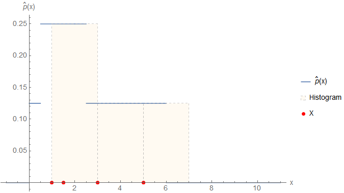
Figure 2: Estimate \(\hat{p}(x)\) calculated using \eqref{eq:ParzenWindow_KernelDensity} with \(h=2\) and the uniform kernel \(K_U(x)\) from \eqref{eq:ParzenWindow_KernelUniform}. The histogram from before is drawn in the background for comparison. The data points are visualized as red points on the \(x\)-axis.
Even though the two PDFs are not identical, they are very similar in the sense that both are step functions, i.e. not smooth. This is the case because \eqref{eq:ParzenWindow_KernelDensity} inherits its properties from the underlying kernels: uniform kernels are not smooth and the same is true for \(\hat{p}(x)\).
So much for the detour to uniform kernels. Hopefully, this has helped to understand the intuition behind \eqref{eq:ParzenWindow_KernelDensity}. Things get even more interesting when we start using a more sophisticated kernel; a Gaussian kernel for instance (with mean \(\mu\) and standard deviation \(\sigma\))
This kernel choice makes the Parzen estimator more complex but is also a requirement to achieve our smoothness constraint. The good thing is, though, that our recent findings remain valid. If we use this kernel in \eqref{eq:ParzenWindow_KernelDensity} with our example data \(X\) (\eqref{eq:ParzenWindow_ExampleData}), we end up with
Even though the function is now composed of more terms, we can still see the individual Gaussian functions and how they are placed at the locations of the data points. The interesting thing with the standard Gaussian kernel \(K_g(x)\) is that the shift \(x_i - x\) and the parameter \(h\) correspond directly to the mean \(\mu\) and the standard deviation \(\sigma\) of the non-standard Gaussian function \(g(x)\). You can see this by comparing \eqref{eq:ParzenWindow_Gaussian} with \eqref{eq:ParzenWindow_EstimateGaussian} which basically leads to the following assignments:
\begin{align*}
\mu &= x_i \\
\sigma &= h
\end{align*}
i.e. the Gaussian kernel is scaled by \(h\) and shifted to the position of \(x_i\). How does \(\hat{p}(x)\) now look like and what is the global effect of the side length \(h\)? You can find out in the following animation.
Figure 3: Estimation of \(\hat{p}(x)\) (blue) by using the Parzen window estimator (\eqref{eq:ParzenWindow_KernelDensity}) with Gaussian kernels applied to the example data \(X\) (\eqref{eq:ParzenWindow_ExampleData}). Besides the PDF itself, you can also visualize the corresponding histogram and the Gaussian kernels. The former is calculated according to \eqref{eq:ParzenWindow_Histogram} and the bins are set to occupy the relevant area. Note that the kernels are manually scaled-down to be visible in this plot: \(\tilde{K}_G(x) = 0.1 \cdot K_g\left(\xfrac{x_i - x}{h}\right)\). Use the slider to control the bin width \(h\) and see how it influences the resulting PDF, the histograms and the kernels.
Note how (as before) each kernel is centred at the position of the data points and that the side length \(h\) still influences how many points are aggregated. But compared to the uniform kernels before, we don't have the clear endings of the bins anymore. It is only noticeable that the Gaussians get wider. However, this is exactly what makes our resulting function smooth and this is, after all, precisely what we wanted to achieve in the first place.
Before we move further to an example in the two-dimensional case, let us make a small detour and reach the Parzen window estimator from a different point of view: convolution.
If you asked a specialist from the signal theory field about the Parzen window estimator, you would probably get a different explanation which includes the words “convolution” and “delta functions”. Even though this approach is completely different from what we have so far, the result still coheres with our previous findings. The first thing we need to do is to convert our data points to a continuous function \(s(x)\) (the input signal). We can do so by placing a Dirac delta function \(\delta(x)\) at each data point
As you can see, the response is already the estimate \(\hat{p}(x)\) and the result is indeed the same as in \eqref{eq:ParzenWindow_EstimateGaussian}. Note that the shifting \(x_i - x\) is not necessary anymore since this part is already handled by the delta functions. An important aspect to mention here is the identity property of the convolution operation: if you convolve a function with the delta function, you get again the input function in return. This property applied to the kernel means
and that explains how the kernels are shifted to the positions of the data points. To see how the response emerges “over time”, you can check out the following animation.
Figure 4: Estimation of \(\hat{p}(x)\) (blue) via convolution. The bin width is set to \(h=1\). With the parameter \(t\), you can control the convolution process, i.e. show the response only for \(x \leq t\). The kernel functions are scaled to the height of the visual representation of the delta functions6 and they are centred exactly at the positions of the delta functions because of \eqref{eq:ParzenWindow_ConvolutionIdentity}.
Of course, the responses are also visually identical. This is not surprising since the same function is plotted. If you take the time, you can see why the resulting function looks the way it does. For example, around \(t=1.5\), the PDF \(\hat{p}(x)\) reaches its maximum. This becomes clear if you consider the kernel functions around this position: when approaching \(t=1.5\) from the left side, two Gaussians are rising (orange and green) and one is falling (blue). After \(t=1.5\) only one function is rising (green) and two are falling (blue and orange). Hence, the summed kernel responses must also decrease after \(t=1.5\).
So much for the detour to the convolution approach. It is interesting to see that both approaches lead to the same result and in essence cover the same idea (but implemented differently): use a set of kernel functions to generate a PDF which reflects the distribution of the data points. The next step is to generalize \eqref{eq:ParzenWindow_KernelDensity} to arbitrary dimensions and give an example in the two-dimensional case.
Extending \eqref{eq:ParzenWindow_KernelDensity} to work in arbitrary dimensions is actually pretty simple. The idea is that our bin, which we assumed so far as a structure which expands only in one dimension, is now a hypercube7 expanding to arbitrary dimensions. This results in a quad in 2D and a cube in 3D. Nevertheless, the general idea is always the same: collect all the data which falls into the hypercube, i.e. lies inside the boundaries of the hypercube. Note that this is also true if you want to calculate a histogram of higher dimensional data.
The factor \(\xfrac{1}{h}\) in \eqref{eq:ParzenWindow_KernelDensity} (or \eqref{eq:ParzenWindow_Histogram}) has compensated for the bin width so fare. When we want to use hypercubes, we must compensate by the hypervolume instead (area in 2D, volume in 3D etc.). So, the only adjustment in order to work in the \(d\)-dimensional space is to divide by \(\xfrac{1}{h^d}\) instead. This leads to the generalization of \eqref{eq:ParzenWindow_KernelDensity}:
Definition 2: Kernel density estimation (Parzen window estimation) [\(d\)-dimensional]
Let \(X = \left( \fvec{x}_1, \fvec{x}_2, \ldots, \fvec{x}_N \right) \in \mathbb{R}^{N \times d}\) be the matrix containing the \(d\)-dimensional data points \(\fvec{x}_i \in \mathbb{R}^d\) (\(i\)-th row of \(X\)). Each column corresponds to a variable (or feature) and each row to an observation. Then, we can use the Parzen window estimator
to retrieve a valid PDF which returns the probability density for \(d\) independent variables \(\fvec{x} = \left( x_1, x_2, \ldots, x_d\right)\). The kernels \(K(x)\) have to be valid PDFs and are parametrized by the side length \(h \in \mathbb{R}^+\).
The only new parameter is the dimension\(d\). The other difference is that the independent variable \(\fvec{x} = (x_1, x_2, \ldots, x_d)\) is now a vector instead of a scalar since \(\hat{p}(\fvec{x})\) produces a multi-dimensional PDF. In the following tab pane, you can see an example in the two-dimensional case.
Figure 6: Two-dimensional estimate \(\hat{p}(\fvec{x})\) generated via \eqref{eq:ParzenWindow_KernelDensity2D} applied to the example data of the first tab. Besides the side length \(h\), you can also switch between three different kernels which are also plotted in the third tab.
Figure 7: Plots of the kernels which are used by the estimator. For the definition of the kernel functions see the attached Mathematica notebook or the documentation of the SmoothKernelDistribution[] function. Note that there is no specific reason for using these three kernels. The intention is to allow to play around and observe the effect of different kernel functions.
Did you notice that the range of \(h\) had been \([0.2;2.5]\) in the first and \([0.05;0.5]\) in the second example? You may noticed that setting \(h\) to the same value does necessarily lead to the same results. Of course, we cannot expect identical PDFs since the data points and even the dimensionality is different. However, even when we bear in mind these differences, the resulting functions are still not the same. More precisely, smaller values for \(h\) in the first example are sufficient to get a smooth function. This is because the scaling of the data is different in both cases. Hence, \(h\) should be selected whilst taking into account the scaling of the data. This is also intuitively clear: the width (or hypervolume) of the bins is spanned in the space of the data and hence inherits its scaling. It is therefore not possible to give general recommendations for the parameter \(h\). However, there are different heuristics to get estimates for this parameter8.
We have now finished our discussion about the Parzen window estimator. We started to define what a good PDF is composed of (resemble the data, smoothness and validity) and then approached the goal in two ways. One way led over histograms which are simplistic PDFs by themselves but can be extended to also fulfil the smoothness constraint. However, even this extension (the Parzen window estimator) inherits the basic behaviour and ideas from the histograms; namely the bins which collect the data and are parametrized by the side length \(h\). Depending on the kernel \(K(x)\), these bins may not have strictly defined borders. The other way led to the signal theory where we transferred our data points to a superposition of delta functions which we then simply convolved with the kernel and we saw that the two ways lead to identical results. In the last part, we generalized the approach to arbitrary dimensions and took a look at a two-dimensional example.
List of attached files:
ParzenWindow.nb [PDF] (Mathematica notebook which contains all the one-dimensional examples and graphics)
When you have worked with images in OpenCL before, you may have wondered how to store them. Basically, we have the choice between using buffers or image objects. The later seems to be designed for that task, but what are the differences and how do they perform differently when applying a certain task? For a recent project, I needed to decide which storage type to use and I want to share the insights here. This is a follow-up article to my previous post where I already evaluated filter operations in OpenCL.
I did not only need to store plain images but rather a complete image pyramid, like visualized in the following figure, originating from a scale space. The pyramid consists of four octaves with four images each making up 16 levels in total. In each octave, the size of the images is always the same. With my used example image, the four images in the first octave have the size of the base image which is \(3866 \times 4320\) pixels. \(1933 \times 2160\) pixels are used in the second, \(966 \times 1080\) in the third and \(483 \times 540\) in the fourth octave making up a total of 88722000 pixels.
Figure 1: Image pyramid consisting of four octaves with four images each. The image is half-sampled after each octave.
In order to measure the performance for the best storage types to use for the image pyramid, I applied image convolution with two derivative filters (Scharr filters) to the complete pyramid testing with the filter sizes of \(3 \times 3\),\(5 \times 5\), \(7 \times 7\) and \(9 \times 9\). I decided to assess four storage types for this task:
Buffer objects are basically one-dimensional arrays which can store any data you want. All pixel values of the image pyramid are stored as a one-dimensional array with a length of 88722000 in this case. This introduces overhead in the access logic, though, since the pyramid is by its nature not one-dimensional but rather three-dimensional with a non-uniform structure, i.e. not all images in the pyramid have the same size. I use a lookup table to minimize the overhead during computation. However, there is still the overhead for the programmer which needs to implement the logic.
Image buffer objects are created from buffers (so a cl::Buffer object is additionally necessary on the host side) and are offered by convenience to use a buffer which behaves like an image. However, it is very limited and can e.g. not be controlled by a sampler object. But it turns out that it is sometimes faster than buffers on my machine as we will see later. In theory, it would also be possible to use one-dimensional images (e.g. image1d_t in the kernel code) but this type of object is limited to the maximum possible width of a 2D image object (16384 on my machine) and hence not suitable to store an image pyramid with 88722000 pixels. Image buffers are not under this constraint but rather restricted by the CL_DEVICE_IMAGE_MAX_BUFFER_SIZE value (134217728 on my machine).
Images are a special data type in OpenCL which can be one-, two- and three-dimensional. The 16 levels of the image pyramid are stored as 16 image objects, e.g. as std::vector<cl::Image2D>. Handling of this object type is easiest for the programmer and as it will turn out is also very fast and I ended up using this storage type for my project.
Cubes are very similar to image types. They basically add a third dimension to the image objects. The idea here is that each octave, where all images have the same size, is stored in one cube resulting in four cubes in total. The overhead should be less for cubes than for images but I could not confirm this definitively in the benchmarks below hence I did not use this type.
The idea behind the four storage types is also visualized in the following figure.
Figure 2: Four different storage types (buffer/image buffer, images and cubes) used in this benchmark. The first quads (buffers) represent pixels, the other images.
The four types and their properties are also summarized in the table below.
The column with the kernel calls denotes how often the OpenCL kernel must be executed in order to apply one filter to the complete image pyramid. Images need the most since the filter kernel must be applied to each image layer in the pyramid individually. The other types contain the notion of an octave in the pyramid and hence know that four images have the same size. It is, therefore, possible to apply the filter function to the complete octave at once.
Before diving into the benchmark though, I want to describe a bit the hardware details about the differences between buffers and images. Note that I use an AMD R9 290 @ 1.1 GHz GPU in the benchmark and hence concentrate only on the GCN architecture.
It is not very easy to find detailed information about how the different storage types are handled by the hardware (or I am too stupid to search). But I will present my findings anyway.
The most important note is that image objects are treated as textures in the graphics pipeline. Remember that GPUs are designed for graphics tasks and the thing we do here in GPGPU with OpenCL is more the exception than the rule (even though it is an important field). Textures are a very important part of computer graphics and when you have ever developed your own (min)-game you know how fruitful this step is. As soon as textures are involved the whole scene does look suddenly much better than before. It is therefore only natural that the hardware has native support for it.
In computer graphics, a lot of tasks need to be done related to textures, e.g. texture mapping. This is the process where your images are mapped to the triangles in the scene. Hence, the hardware needs to load the necessary image pixels, maybe do some type conversion (e.g. float to int) or even compression (a lot of textures need a lot of space) and don't forget address calculations, interpolating as well as out-of border handling. To help with these tasks, the vendors add extra texture units which implement some of the logic in hardware. This is also visible in the block diagram of a compute unit of the AMD R9 290
As you can see, the transistors responsible for textures are located on the right side. There are four texture units (green horizontal bars) where each unit is made up of one filter unit and four address units. Why four times more address units than filter units? I don't know if this was the design choice but I would guess that this has something to do with bilinear interpolation where four pixels are needed to calculate one texel. It is also possible that this has something to do with latency hiding and hardware parallelism. Memory fetches may need a lot of time compared to the execution of ALU instructions in the SIMD units. In order to stay busy, the hardware executes multiple threads at once so that while one thread still waits for the data the others can already start with execution. But each thread needs data and must issue memory requests hence multiple store and load units are necessary. Note that these texture units are located on each compute unit and are not shared on a per-device basis. My device has 40 compute units so there are 160 texture units in total.
The address units take the requested pixel location, e.g. an \(x\) and \(y\) coordinate, and calculate the corresponding memory address. It could be possible that they do something like \(cols*y + x\) to calculate the address. When interpolation is used, the memory addresses for the surrounding pixels must be calculated as well. Anyway, requests to the memory system are issued and this involves the L1 cache (16 KB) next to the address units. This cache is sometimes also called the texture cache (since it holds texels).
Since the cache is shared between all wavefronts on the compute unit, it offers an automated performance gain when the wavefronts work on overlapping regions of the same data. E.g. in image convolution the pixels need to be accessed multiple times due to the incorporation of the neighbourhood. When the wavefronts on the compute unit process neighbouring image areas, this can speed up the execution since less data needs to be transferred from global to private memory. It is loaded directly from the cache instead.
There is also a global L2 texture cache with a size of 1 MB which is shared by all compute units on the device. Usually, the data is first loaded in the L2 cache before it is passed to the L1 caches of the compute units. In case of image convolution, the L2 cache may hold a larger portion of the image and each compute unit uses one part of this portion. But there is an overlap between the portions since pixels from the neighbourhood are fetched in the image convolution operation as well.
Buffers and image objects are also accessed differently from within OpenCL kernel code. Whereas a buffer is only a simple pointer and can be accessed as (note also how the address calculation is done in the kernel code and hence executed by the SIMD units)
kernel void buffer(global float* imgIn, global float* imgOut, const int imgWidth)
{
    const int x = get_global_id(0);
    const int y = get_global_id(1);
    float value = imgIn[imgWidth * y + x];
    //...
    imgOut[imgWidth * y + x] = value;
}
i.e. directly without limitations (it is just a one-dimensional array), image objects need special built-in functions to read and write values:
// CLK_ADDRESS_CLAMP_TO_EDGE = aaa|abcd|ddd
constant sampler_t sampler = CLK_NORMALIZED_COORDS_FALSE | CLK_ADDRESS_CLAMP_TO_EDGE | CLK_FILTER_NEAREST;

kernel void images(read_only image2d_t imgIn, write_only image2d_t imgOut)
{
    const int x = get_global_id(0);
    const int y = get_global_id(1);
    float value = read_imagef(imgIn, sampler, (int2)(x, y)).x;
    //...
    write_imagef(imgOut, (int2)(x, y), value);
}
So, the function read_imagef(image2d_t image, sampler_t sampler, int2 coordinates) is needed to access the pixels. This is necessary so that the hardware can optimize the code and make use of the texture units where the sampler is used to configure it. But how can the cool functions I promised before now be used in OpenCL or equivalently: how to set up the texture filter units to do what we want?
Interpolating: set the sampler to CLK_FILTER_LINEAR for bilinear and CLK_FILTER_NEAREST for nearest neighbour filtering. The additional texels are loaded automatically and the interpolated value is returned. If you need this interpolating functionality, you can also store other data than pixels in the image objects and get automatic interpolation.
Out-of-border handling: set the sampler e.g. to CLK_ADDRESS_CLAMP_TO_EDGE to repeat the last values or use one of the other constants. The modes are a bit limited when not using normalized coordinates, though; but still, better than nothing.
Type conversion: this is controlled by the used function in the kernel. Above read_imagef was used which returns a float value. Use e.g. read_imagei to return an int. Note that the functions in the kernel are independent of the real format set up on the host side.
How do buffer objects now differ? They don't use the texture units for a start since we do not provide a sampler object and do not use the built-in access functions. But they also use the cache hierarchy (bot L1 and L2) according to the docs. The programming guide by AMD states on page 9 “Actually, buffer reads may use L1 and L2. [...] In GCN devices, both reads and writes happen through L1 and L2.” and in the optimization guide on page 14 they claim further “The L1 and L2 read/write caches are constantly enabled. Read-only buffers can be cached in L1 and L2.”. This sounds for me that both caches are used for buffers as well but the benchmark results below suggest that a cache-friendly local work-group size seems to be important.
Regarding performance of the different memory locations, the general relationship is global > texture cache > local > private (cf. page 13ff of the optimization guide for some numbers). So even when image objects and hence texture cache is used, it may still be beneficial to explicitly cache data which is needed more than once by using the local data share (located in the centre in the block diagram). It is not surprising that global memory is the slowest and private memory the fastest. The trick is to reduce the time needed to transfer the data in the private registers of the SIMD units.
The buffer object is stored as a very long array in memory, but we still need to access locations in one of the images of the pyramid. But when we have only access to the 1D array from within the kernel, how do we write to a certain pixel location, let's say point \(p_1 = (10, 2)\) in level 9 of the pyramid? I decided to use a lookup table which is implemented as an array of structs defined as
struct Lookup
{
    int previousPixels;
    int imgWidth;
    int imgHeight;
};
The most important information is previousPixels which gives the number of pixels from all previous images and hence is the start offset for the buffer to find the pixel in the considered image. Helper functions to read and write to a certain pixel location can now be defined as
float readValue(float* img, constant struct Lookup* lookup, int level, int x, int y)
{
    return img[lookup[level].previousPixels + lookup[level].imgWidth * y + x];
}

void writeValue(float* img, constant struct Lookup* lookup, int level, int x, int y, float value)
{
    img[lookup[level].previousPixels + lookup[level].imgWidth * y + x] = value;
}
E.g. for \(p_1\) the memory address is calculated as lookup[8].previousPixels + lookup[8].966 /* = 3866 / 4 */ * 2 + 10. The lookup array is filled on the host side and transferred to the GPU as an argument to the filter kernel. The following snippet does the computation on the host side and includes an example.
/*
 * The following code generates a lookup table for images in a pyramid which are located as one long
 * buffer in memory (e.g. 400 MB data in memory). The goal is to provide an abstraction so that it is
 * possible to provide the level and the pixel location and retrieve the image value in return.
 *
 * Example:
 *  - original image width = 3866
 *  - original image height = 4320
 *  - image size in octave 0 = 3866 * 4320 = 16701120
 *  - image size in octave 1 = (3866 / 2) * (4320 / 2) = 4175280
 *  - image size in octave 2 = (3866 / 4) * (4320 / 4) = 1043820
 *  - number of octaves = 4
 *  - number of images per octave = 4
 *
 *  Number of pixels for image[8] (first image of octave 2):
 *  - pixels in previous octaves = 4 * 16701120 + 4 * 4175280 = 83505600
 *  - previous pixels for image[8] = 83505600
 *
 *  Number of pixels for image[9] (second image of octave 2):
 *  - pixels in previous octaves = 4 * 16701120 + 4 * 4175280 = 83505600
 *  - previous pixels for image[9] = 83505600 + 1043820 = 84549420
 */
locationLoopup.resize(pyramidSize);
int previousPixels = 0;
int octave = 0;
for (size_t i = 0; i < pyramidSize; ++i)
{
    locationLoopup[i].previousPixels = previousPixels;

    // Store size of current image
    locationLoopup[i].imgWidth = static_cast<int>(img.cols / pow(2.0, octave));
    locationLoopup[i].imgHeight = static_cast<int>(img.rows / pow(2.0, octave));

    // The previous pixels for the next iteration include the size of the current image
    previousPixels += locationLoopup[i].imgWidth * locationLoopup[i].imgHeight;

    if (i % 4 == 3)
    {
        ++octave;
    }
}
The same technique is used for the image buffers as well. When it comes to enqueue the kernel at the host side, the following code is executed for each octave.
//...
const size_t depth = 4;
const int base = octave * depth;    // octave is given as function argument
const size_t rows = lookup[base].imgHeight;
const size_t cols = lookup[base].imgWidth;

//...
const cl::NDRange offset(0, 0, base);
const cl::NDRange global(cols, rows, depth);
queue->enqueueNDRangeKernel(kernel, offset, global, local);
Note the used offset which stores the number of previous images (e.g. 8 in the octave = 2 iteration) and depth = 4 which makes this kernel a 3D problem: the filter is computed for all image pixels in all four images of the current octave.
The code for images and cubes is not very exciting, so I will not show any details for them. Check out the implementation if you want to know more.
It is now time to do some benchmarking. I start by testing a normal filter operation (called single in the related article). A short summary of the implementation is: unrolling and constant memory is used for the filter but no other optimizations. The first thing I want to test is the difference between the default local work-group size, i.e. setting the corresponding parameter to cl::NullRange, and the size manually to \(16 \times 16\). This is a common block size for an image patch computed by a work-group and is also the maximum possible size on my AMD R9 290 GPU. It turns out that this setting is quite crucial for buffers as you can see in the next figure.
Figure 3: Benchmark which tests the influence of the local work-group size (but not using local memory yet). Default settings (solid) are compared to a fixed size of \(16 \times 16\) (dashed). Note that this is the maximum possible size for a work-group on an AMD R9 290. Hover over the points to see the exact number. Click on the label at the top to hide/show a line (especially useful for the buffer to make space for the other lines). The mean values per size are averaged over 20 runs. Test suite used to produce these numbers is also available on GitHub
It really is important to manually set the local work-group size for buffers. Performance totally breaks for larger filters. The fact that a fixed size increases the speed that much is, I think, indeed evidence that buffers use the cache hierarchy. Otherwise, the local size shouldn't matter that much. But, there are still some differences compared to image buffers. Even though they also profit from a manually set work-group size, the effect is not that huge. Maybe the texture address units do some additional stuff not mentioned here which helps to increase cache performance. I don't think that it is related to some processing in the texture filter units since there is not much left. No type conversion must be done and a sampler can't be used for image buffers anyway. Additionally, the address calculation (\(cols*y + x\)) is done in both buffers inside the kernel and therefore executed by the SIMD units. Another possibility would be that the local work-group size is set differently for image buffers than for normal buffers. Unfortunately, I don't know of a way to extract this size when not set explicitly (the profiler just shows NULL).
If you compare the image buffers with one of the other image types (e.g. images), you see that image buffers are a bit slower. This is the effect of the missing sampler and the address calculation which needs to be done manually for image buffers. So, if possible, you should still prefer the normal image type over image buffers. But let me note that sometimes it is not possible or desired to work with 2D image objects. For example, let's say you have a point structure like
struct KeyPoint
{
    int octave;
    int level;
    float x;
    float y;
};
and you want to store a list of points which can be located anywhere in the image pyramid. Suppose further you want later (e.g. in a different kernel call) access the image pixels and its neighbours. Then you need to have access to the complete image pyramid inside the kernel and not only to a specific image. This is only possible when the pyramid is stored in an (image) buffer because then you can read pixels from all levels at once.
Another noticeable comparison is between images and cubes. First, the local work-group size does not play an important role in both cases. The differences here are negligible. It is likely that the hardware has more room for optimization since it knows which pixels in the 2D image plane are accessed. Remember that bot \(x\) and \(y\) are provided to the access functions. Second, cubes are consistently slower than images. Even though cubes can be executed with only 4 instead of 16 kernel calls and hence results in less communication with the driver and therefore less overhead. Maybe cubes are too large and stress the caches too much so that the benefit of the kernel calls are neutralized. Anyway, this is precisely the reason why I decided to use images and not cubes to store my pyramid.
The next thing I want to assess is the benefit of local memory. The following chart compares the results for fixed size work-groups from before with the case that always local memory is used (implementation details about how to use local memory for this task are shown in the filter evaluation article).
Figure 4: Benchmark which tests the usage of local memory. With local (solid) is compared against no usage of local memory (dashed). In both cases, the local work-group size is set to a fixed size of \(16 \times 16\). Note that the dashed values are the same as in the previous chart and are just shown again for comparison. Hover over the points to see the exact number. Click on the label at the top to hide/show a line. The mean values per size are averaged over 20 runs.
It is clear that local memory is beneficial for filter sizes \(\geq 5 \times 5\) regardless of the storage type. This is not surprising though since local memory is still faster than the L1 cache. Additionally, the L1 cache is smaller (16 KB L1 vs. 64 KB LDS), so it is to be expected that for larger filters performance decreases. For a filter of size \(3 \times 3\) the situation is not that clear. Sometimes it is faster and sometimes not. Don't forget that the manual caching with local memory does also introduce overhead. The data must be copied to the LDS and read back by the SIMD units. In general, I would say that it is not worth to use local memory for such a small filter.
Considering only the lines which use local memory, the result looks a bit messy. No clear winner and crossings all over again. I decided to use normal image types since they are easy to handle and offer full configuration via the sampler object. But I would also recommend that you test this on your own hardware. The results are very likely to differ.
Filter operations are very common in computer vision applications and are often the first operations applied to an image. Blur, sharpen or gradient filters are common examples. Mathematically, the underlying operation is called convolution and already covered in a separate article. The good thing is that filter operations are very well suited for parallel computing and hence can be executed very fast on the GPU. I worked recently on a GPU-project were the filter operations made up the dominant part of the complete application and hence got first priority in the optimization phase of the project. In this article, I want to share some of the results.
First, a few words about GPU programming1. The GPU is very different from the CPU since it serves a completely different purpose (mainly gaming). This results in a completely different architecture and design principles. A GPU is a so-called throughput-oriented device where the goal is to execute many, many tasks concurrently on the processing units. Not only that a GPU has much more processing units than a CPU, it is also designed to leverage massive parallelism, e.g. by the concept of additional hardware threads per core. Just as a comparison: the CPU is a latency-oriented device. Its main goal is to execute a single task very fast, e.g. by introducing fast memory caching mechanism.
The demanding task for the developer is to keep the GPU busy. This is only possible by exploiting the parallelism of the application and optimize the code regarding this subject. One important factor, and as I now learned the important factor, which stalls the GPU is memory access. Since the GPU has a lot of processing units it needs also more memory to serve the units with data. Unlike to the CPU, it is under control of the developer where to store the memory which offers great flexibility and an additional degree of freedom in the optimization process. Badly designed memory transfers, e.g. by repeatedly copying data from the global to the private memory of the work-items, can take up most of the execution time.
As you may already have guessed from the title, I use OpenCL as a framework in version 2.0 and all the tests are run on an AMD R9 2902 @ 1.1 GHz GPU. Scharr filter (gradient filter) in the horizontal and vertical direction
are used as filter kernel (centre position highlighted) and applied to an image pyramid consisting of four octaves with four images each3. Every benchmark measures how fast the two filters can be applied to the complete pyramid averaged over 20 runs. Note, that the creation of the pyramid (including the initial image transfer to the GPU) or the compilation time of the kernels is not included. I only want to measure the impact of the filter operation. Since the size of the filter is also very important, four different dimensions are used: \(3 \times 3\),\(5 \times 5\), \(7 \times 7\) and \(9 \times 9\). Filters larger than \(3 \times 3\) are basically \eqref{eq:FilterOptimization_ScharrFilter} scaled up but with slightly different numbers. In any case, there are only six non-zero entries. Filters are stored in float* arrays and the image itself is a grey-scale image converted to floating data type, i.e. the OpenCL data type image2d_t is used.
I want to assess the performance of filter operations in five test cases:
Single: filter operation without further optimizations.
Local: the image data is cached in local memory to exploit the fact that each pixel is needed multiple times.
Separation: both filters in \eqref{eq:FilterOptimization_ScharrFilter} are linearly separable. In this case, it is possible to split up each filter in a horizontal and vertical vector and apply them to the image in two passes.
Double: \(\partial_x\) and \(\partial_y\) are independent of each other. Since usually the response from both filters is needed and both are applied to the same image, it is possible to write an optimized kernel for that case.
Predefined: Scharr filters are very common and it is likely that we need them multiple times. We could write a specialized kernel just for Scharr filters without the need to pass the filter as a parameter to the kernel. We can even go one step further and take the values of the filter into account, e.g. by omitting zero entries.
I don't have an extra case where I put the filter in constant memory since this is an optimization which I already implemented in the beginning (it is not very hard since the only thing to do is to declare the parameter pointing to the filer as constant float* filter), so the usage of constant memory is always included. Another common optimization is filter unrolling where the filter size must be known at compile time. The compiler can then produce code containing the complete filter loop as explicit steps without introducing the loop overhead (e.g. conditional checks if the loop has ended). Since this is also something where every test case benefits from, it is included, too.
Note also that these cases are not independent of each other. It is e.g. possible to use local memory and separate the filter. This makes testing a bit complicated since there are a lot of combinations possible. I start by considering each case separately and look at selected combinations at the end. All code which I used here for testing is also available on GitHub.
The next sections will cover each of the test cases in more detail, but the results are already shown in the next figure so that you can always come back here to compare the numbers.
Figure 1: Test results for the filter operations as mean value over 20 runs for different filter sizes. Hover over the points to see the exact number. Click on the label at the top to hide/show a line. Don't be too confident with the absolute speed values since they depend highly on the used hardware and maybe also other things like driver version, but the ordinal relationship should be a bit meaningful.
The basic filter operation without any optimizations is implemented straightforwardly in OpenCL. We centre our Scharr filter at the current pixel location and then perform the convolution. The full code is shown as it serves as the basis for the other test cases.
/**
 * Calculates the filter sum at a specified pixel position. Supposed to be called from other kernels.
 *
 * Additional parameters compared to the base function (filter_single_3x3):
 * @param coordBase pixel position to calculate the filter sum from
 * @return calculated filter sum
 */
float filter_sum_single_3x3(read_only image2d_t imgIn,
                            constant float* filterKernel,
                            const int2 coordBase,
                            const int border)
{
    float sum = 0.0);
    const int rows = get_image_height(imgIn);
    const int cols = get_image_width(imgIn);
    int2 coordCurrent;
    int2 coordBorder;
    float color;

    // Image patch is row-wise accessed
    // Filter kernel is centred in the middle
    #pragma unroll
    for (int y = -ROWS_HALF_3x3; y <= ROWS_HALF_3x3; ++y)       // Start at the top left corner of the filter
    {
        coordCurrent.y = coordBase.y + y;
        #pragma unroll
        for (int x = -COLS_HALF_3x3; x <= COLS_HALF_3x3; ++x)   // And end at the bottom right corner
        {
            coordCurrent.x = coordBase.x + x;
            coordBorder = borderCoordinate(coordCurrent, rows, cols, border);
            color = read_imagef(imgIn, sampler, coordBorder).x;

            const int idx = (y + ROWS_HALF_3x3) * COLS_3x3 + x + COLS_HALF_3x3;
            sum += color * filterKernel[idx];
        }
    }

    return sum;
}

/**
 * Filter kernel for a single filter supposed to be called from the host.
 *
 * @param imgIn input image
 * @param imgOut image containing the filter response
 * @param filterKernel 1D array with the filter values. The filter is centred on the current pixel and the size of the filter must be odd
 * @param border int value which specifies how out-of-border accesses should be handled. The values correspond to the OpenCV border types
 */
kernel void filter_single_3x3(read_only image2d_t imgIn,
                              write_only image2d_t imgOut,
                              constant float* filterKernel,
                              const int border)
{
    int2 coordBase = (int2)(get_global_id(0), get_global_id(1));

    float sum = filter_sum_single_3x3(imgIn, filterKernel, coordBase, border);

    write_imagef(imgOut, coordBase, sum);
}
The sampler is a global object. Also, borderCoordinate() is a helper function to handle accesses outside the image border. Both definitions are not shown here and I refer to the full implementation (both are defined in filter.images.cl) for further interest, but it is not important here for the tests. We can call the filter_single_3x3() kernel from the host with the cl::NDRange set to the image size of the current level in the pyramid, e.g. something like
with the half versions calculated with int cast, i.e. \(rowsHalf = \left\lfloor \frac{rows}{2} \right\rfloor\). They need to be set as defines so that #pragma unroll can do its job. As you can see from the test results, this solution is not very fast compared to the others. This is good news since there is still room for optimizations.
In the filter operation, each pixel is accessed multiple times by different work-items due to the incorporation of the neighbourhood in the convolution operation. It is not very efficient to transfer the data again and again from global to private memory since access to global memory is very slow. The idea is to cache the image's pixel values in local memory and access it from here. This reduces the need for global memory transfers significantly.
Local memory is attached to each compute unit on the GPU and is shared between work-groups. Work-groups on different compute units can't share the same data, so the caching is restricted to the current work-group. Since the work-group size is limited, e.g. to \(16 \times 16\) on the AMD R9 290 GPU, we need to split up the image into \(16 \times 16\) blocks. Each work-group must copy the parts of the image it needs into its own local memory. This would be easy if a work-group would only need to access data from its own \(16 \times 16\) image block. But the incorporation of the neighbourhood also holds for the border pixels, so we need to copy a bit more than \(16 \times 16\) pixels from the image depending on the filter size. E.g. for a \(3 \times 3\) filter a 1 px wide padding is needed.
Ok, we just need to copy a few more pixels, shouldn't be a problem, should it? It turns out that this is indeed a bit tricky. The problem is: which work-items in the work-group copy which pixels? We need to define a pattern and write it down as (messy) index calculation in code. To make things a bit simpler, consider the following example of a \(16 \times 16\) block which is located somewhere around the top left corner.
Figure 2: Example for the transfer from global to local memory with a \(3 \times 3\) filter. The outer index (black) corresponds to the image access in the for loop of the next listing. Inside the pixels, the top index \({\color{Orange}(x_{local},y_{local})}\) shows the local id and the bottom index pair \({\color{Green}(x_{global},y_{global})}\) the global id used in this example. Blue pixels are needed for padding to allow correct filter calculations of the border pixels. The green pixel in the top left corner of the patch marks the base pixel.
First, note that the size of the local buffer must be large enough to cover all pixels shown. The idea is then to iterate over the local buffer (outer index), map the calculation relative to the base pixel and then copy the data according to the current outer pixel. Usually, this involves 4 iterations where we start with a \(16 \times 16\) block in the top left corner and move on in a zigzag fashion to gather the remaining pixels as shown in the following figure.
Figure 3: Access pattern of the 2-loop approach which fills the local buffer in four iterations using a \(3 \times 3\) filter.
Except for the first iteration and not too large filter sizes, not all of the 256 work-items are busy during this calculation. Especially the fourth iteration where only 4 of the 256 work-items do something useful is not beautiful to look at4. But since the local buffer size does not map perfectly with the size of the work-group, this is unavoidable with this pattern. Implementing it results in:
/**
 * Calculates the filter sum using local memory at a specified pixel position. Supposed to be called from other kernels.
 *
 * Additional parameters compared to the base function (filter_single_local_3x3):
 * @param coordBase pixel position to calculate the filter sum from
 * @return calculated filter sum
 */
float filter_sum_single_local_3x3(read_only image2d_t imgIn,
                                  constant float* filterKernel,
                                  int2 coordBase,
                                  const int border)
{
    const int rows = get_image_height(imgIn);
    const int cols = get_image_width(imgIn);

    // The exact size must be known at compile time (no dynamic memory allocation possible)
    // Adjust according to the highest needed filter size or set via compile parameter
    local float localBuffer[LOCAL_SIZE_COLS_3x3 * LOCAL_SIZE_ROWS_3x3];   // Allocate local buffer

    int xLocalId = get_local_id(0);
    int yLocalId = get_local_id(1);

    int xLocalSize = get_local_size(0);
    int yLocalSize = get_local_size(1);

    // The top left pixel in the current patch is the base for every work-item in the work-group
    int xBase = coordBase.x - xLocalId;
    int yBase = coordBase.y - yLocalId;

#if COLS_3x3 >= 9 || ROWS_3x3 >= 9
    /*
     * Copy the image patch including the padding from global to local memory. Consider for example a 2x2 patch with a padding of 1 px:
     * bbbb
     * bxxb
     * bxxb
     * bbbb
     * The following pattern fills the local buffer in 4 iterations with a local work-group size of 2x2
     * 1122
     * 1122
     * 3344
     * 3344
     * The number denotes the iteration when the corresponding buffer element is filled. Note that the local buffer is filled beginning in the top left corner (of the buffer)
     *
     * Less index calculation but more memory accesses, better for larger filter sizes
     */
    for (int y = yLocalId; y < yLocalSize + 2 * ROWS_HALF_3x3; y += yLocalSize)
    {
        for (int x = xLocalId; x < xLocalSize + 2 * COLS_HALF_3x3; x += xLocalSize)
        {
            // Coordinate from the image patch which must be stored in the current local buffer position
            int2 coordBorder = borderCoordinate((int2)(x - COLS_HALF_3x3 + xBase, y - ROWS_HALF_3x3 + yBase), rows, cols, border);
            localBuffer[y * LOCAL_SIZE_COLS_3x3 + x] = read_imagef(imgIn, sampler, coordBorder).x;   // Fill local buffer
        }
    }
#else
    /*
     * Copy the image patch including the padding from global to local memory. The local ID is mapped to the 1D index and this index is remapped to the size of the local buffer. It only needs 2 iterations
     *
     * More index calculations but less memory accesses, better for smaller filter sizes (a 9x9 filter is the first which needs 3 iterations)
     */
    for (int idx1D = yLocalId * xLocalSize + xLocalId; idx1D < (LOCAL_SIZE_COLS_3x3 * LOCAL_SIZE_ROWS_3x3); idx1D += xLocalSize * yLocalSize) {
        int x = idx1D % LOCAL_SIZE_COLS_3x3;
        int y = idx1D / LOCAL_SIZE_COLS_3x3;

        // Coordinate from the image patch which must be stored in the current local buffer position
        int2 coordBorder = borderCoordinate((int2)(x - COLS_HALF_3x3 + xBase, y - ROWS_HALF_3x3 + yBase), rows, cols, border);
        localBuffer[y * LOCAL_SIZE_COLS_3x3 + x] = read_imagef(imgIn, sampler, coordBorder).x;   // Fill local buffer
    }
#endif

    // Wait until the image patch is loaded in local memory
    work_group_barrier(CLK_LOCAL_MEM_FENCE);

    // The local buffer includes the padding but the relevant area is only the inner part
    // Note that the local buffer contains all pixels which are read but only the inner part contains pixels where an output value is written
    coordBase = (int2)(xLocalId + COLS_HALF_3x3, yLocalId + ROWS_HALF_3x3);
    int2 coordCurrent;
    float color;
    float sum = 0.0f;

    // Image patch is row-wise accessed
    #pragma unroll
    for (int y = -ROWS_HALF_3x3; y <= ROWS_HALF_3x3; ++y)
    {
        coordCurrent.y = coordBase.y + y;
        #pragma unroll
        for (int x = -COLS_HALF_3x3; x <= COLS_HALF_3x3; ++x)
        {
            coordCurrent.x = coordBase.x + x;
            color = localBuffer[coordCurrent.y * LOCAL_SIZE_COLS_3x3 + coordCurrent.x];    // Read from local buffer

            const int idx = (y + ROWS_HALF_3x3) * COLS_3x3 + x + COLS_HALF_3x3;
            sum += color * filterKernel[idx];
        }
    }

    return sum;
}
The relevant part is located at the lines 46–54. Notice how x - COLS_HALF_3x3 maps to the outer index shown in the example and when this is added to the base pixel we cover the complete local buffer. For example, the work-item \(w_1 = {\color{Orange}(0, 0)}\) executes the lines in its first iteration as
which copies the top left pixel to the first element in the local buffer. Can you guess which second pixel the same work-item copies in its second iteration?5
When working with local buffers there is one caveat: the size of the buffer must be known at compile time and it is not possible to allocate it dynamically. This means that the defines
must be set properly before using this function. This becomes less of a problem when loop unrolling is used (like here) since then the filter size must be known anyway.
Skip the second #else pragma for now and consider line 76ff where the base index is calculated. This adds the padding to the local id since we need only calculate the filter responses of the inner block (the padding pixels are only read, not written). For example, the work-item \(w_1\) sets this to
and accesses later the top left pixel in its first iteration (since the filter is centred at \({\color{Orange}(0, 0)}\))
// Image patch is row-wise accessed
#pragma unroll
for (int y = -1; y <= 1; ++y)
{
    coordCurrent.y = 1 + -1;
    #pragma unroll
    for (int x = -1; x <= 1; ++x)
    {
        coordCurrent.x = 1 + -1;
        float color = localBuffer[0 * 18 + 0];    // Read from local buffer

        const int idx = (-1 + 1) * 3 + -1 + 1;
        sum += color * filterKernel[0];
    }
}
The access pattern shown in the lines 46–54 has the disadvantage that it needs at least 4 iterations even though a \(3 \times 3\) filter can theoretically fetch all data in two iterations (256 inner pixels and \(16*1*4 + 1*1*4 = 68\) padding pixels). Therefore, I also implemented a different approach (lines 61–68). The idea here is to map the index range of the local ids of the \(16 \times 16\) block to a 1D index and then remap them back to the local buffer size. This is also visualized in the following figure.
Figure 4: Remapping of a \(16 \times 16\) block to the local buffer size of \(18 \times 18\) (\(3 \times 3\) filter). The block indices are mapped to the \(0, \ldots, 255\) 1D index range and remapped back to the indices of the \(18 \times 18\) local buffer size. In the first iteration the opaque pixels are loaded and in the second iteration the transparent pixels (remaining pixels).
For the work-item \(w_{18} = {\color{Orange}(1, 1)}\) lines 61–68 expand to
for (int idx1D = 1 * 16 + 1 /* = 17 */; idx1D < (18 * 18 /* = 324 */); idx1D += 16 * 16 /* = 256 */) {
    int x = 17 % 18 /* = 17 */;
    int y = 17 / 18 /* = 0 */;

    // Coordinate from the image patch which must be stored in the current local buffer position
    int2 coordBorder = borderCoordinate((int2)(17 - 1 + 32, 0 - 1 + 32) /* = (48, 31) */, rows, cols, border);
    localBuffer[0 * 18 + 17] = read_imagef(imgIn, sampler, coordBorder).x;   // Fill local buffer
}
and issues a copy operation for the top right pixel from global memory into the local buffer. Even though this approach results in fewer iterations it comes at the cost of higher index calculations. Comparing the two approaches shows only a little difference in the beginning.
Figure 5: Test results for two different patterns of how to copy the data from global to local memory as mean value over 20 runs for different filter sizes. The blue line shows the result using 2 for loops (lines 46–54) and the orange line denotes the results when using just 1 for loop but more index calculations (lines 61–68).
Only for a \(7 \times 7\) filter there is a small advantage of \(\approx 1.5\,\text{ms}\) for the index remapping approach. It is very noticeable though that a \(9 \times 9\) filter is much faster in the 2-loops approach. This is the first filter which needs 3 iterations in the remapping approach (256 inner pixels and \(16*4*4+4*4*4=320>256\)) and the critical point where the overhead of the index calculations gets higher than the cost of the additional iteration in the 2-loop approach.
Even though the difference is not huge, I decided to use the remapping approach for filter sizes up to \(7 \times 7\) and the 2-loop approach otherwise (hence the #if pragma).
Comparing the use of local memory with the other test cases shows that local memory gets more efficient with larger filter sizes. In the case of a \(3 \times 3\) filter the results are even a little bit worse due to the overhead of copying the data from global to local memory. But for the other filter sizes, this is definitively an optimization we should activate.
Separation is an optimization which does not work with every filter. To apply this technique, it must be possible to split up the filter in one column and one row vector so that their outer product results in the filter again, e.g. for a \(3 \times 3\) filter the equation
How does this help us? Well, we can use this when performing the convolution operation with the image \(I\)
\begin{equation*}
I * \partial_x = I * \fvec{\partial}_{x_1} * \fvec{\partial}_{x_2} = I * \fvec{\partial}_{x_2} * \fvec{\partial}_{x_1}.
\end{equation*}
So, we can perform two convolutions instead of one and the order doesn't matter. This is interesting because we now perform two convolutions with a \(3 \times 1\) respectively a \(1 \times 3\) filter instead of one convolution with a \(3 \times 3\) filter. The benefit may be not so apparent for such a small filter but for larger filters, this gives us the opportunity to save a lot of computations. However, we also increase the memory consumption due to the need for a temporary image which is especially crucial on GPUs, as we will see.
But first, let's look at a small example. For this, consider the following definition of \(I\)
These are our temporary values where we would need a temporary image with the same size as the original image during the filter process. Next, apply the column vector on the previous results
and we get indeed the same result. If you want to see the full example, check out the attached Mathematica notebook.
The kernel code which implements separate filter convolution is not too different from the single approach. It is basically the same function, just using different defines
and adjust the names in the kernel definition accordingly
float filter_sum_single_1x3(read_only image2d_t imgIn,
                            constant float* filterKernel,
                            const int2 coordBase,
                            const int border)
{
    //...
    #pragma unroll
    for (int y = -ROWS_HALF_1x3; y <= ROWS_HALF_1x3; ++y)       // Start at the top left corner of the filter
    {
        coordCurrent.y = coordBase.y + y;
        #pragma unroll
        for (int x = -COLS_HALF_1x3; x <= COLS_HALF_1x3; ++x)   // And end at the bottom right corner
        {
            //...
            const int idx = (y + ROWS_HALF_1x3) * COLS_1x3 + x + COLS_HALF_1x3;
            sum += color * filterKernel[idx];
        }
    }

    return sum;
}
But from the host side, we need to call two kernels, e.g. something like
Note the temporary image imgTmp which serves as output in the first call and as input in the second call. Beside that also two filters are needed at the host side (bufferKernelSeparation1A respectively bufferKernelSeparation1A) there is nothing special here.
If you look at the test results, you see that this approach performs not very well. For a \(3 \times 3\) filter it turns out that this is even a really bad idea since it produces the worst results from all. Even when things get better for larger filter sizes (which is expected) the results are not overwhelming. The main problem here is the need for an additional temporary image. We need as much as the size of the complete image as additional memory. What is more, we have more memory transfers: in the first run the data is transferred from global to private memory, the temporary response calculated and stored back in global memory. In the next run, the data is transferred again from global to private memory to calculate the final response which is, again, stored back in global memory. Since memory transfers from global to private memory are very costly on the GPU this back and forth introduces an immense overhead and this overhead manifests itself in the bad results.
Another thing I noticed here is that the range of values is very high (remember that the test results show only the mean value over 20 runs). This can be seen by considering a box-whisker plot of the data as in the following figure.
Figure 6: Test results for the separation test case shown as box-whisker plot for different filter sizes. The whiskers are set depending on the interquartile range, e.g. for the top whisker: \(q_{75} + 1.5 \cdot (q_{75} - q_{25})\) if an outlier exists. Disable the outlier in the legend to see the box-whisker plots in more detail.
Especially for the \(3 \times 3\) filter the range is really immense with outliers around 500 ms (half a second!). This really breaks performance and may be another symptom of the temporary image. I did not notice such behaviour for the other test cases.
I recently worked on a project where I needed a lot of filter operations which were, theoretically, all separable with sizes up to \(9 \times 9\). In the beginning, I used only separable filters without special testing. Later in the optimization phase of the project, I did some benchmarking (the results you are currently reading) and omitted separable filters completely as a consequence. This was a huge performance gain for my program. So, be careful with separable filters and test if they really speed up your application.
Suppose you want to calculate the magnitude of the image gradients \(\left\| \nabla I \right\|\) (which is indeed a common task). Then both filters of \eqref{eq:FilterOptimization_ScharrFilter} need to be applied to the image and a task graph could look as follows.
Figure 7: Task graph to calculate the magnitude of the image gradients.
As you can see, the two filter responses can be calculated independently from each other. What is more: they both use the same image as input. We can exploit this fact and write a specialized kernel which calculates two filter responses at the same time.
float2 filter_sum_double_3x3(read_only image2d_t imgIn,
                             constant float* filterKernel1,
                             constant float* filterKernel2,
                             const int2 coordBase,
                             const int border)
{
    float2 sum = (float2)(0.0f, 0.0f);
    const int rows = get_image_height(imgIn);
    const int cols = get_image_width(imgIn);
    int2 coordCurrent;
    int2 coordBorder;
    float color;

    // Image patch is row-wise accessed
    // Filter kernel is centred in the middle
    #pragma unroll
    for (int y = -ROWS_HALF_3x3; y <= ROWS_HALF_3x3; ++y)       // Start at the top left corner of the filter
    {
        coordCurrent.y = coordBase.y + y;
        #pragma unroll
        for (int x = -COLS_HALF_3x3; x <= COLS_HALF_3x3; ++x)   // And end at the bottom right corner
        {
            coordCurrent.x = coordBase.x + x;
            coordBorder = borderCoordinate(coordCurrent, rows, cols, border);
            color = read_imagef(imgIn, sampler, coordBorder).x;

            const int idx = (y + ROWS_HALF_3x3) * COLS_3x3 + x + COLS_HALF_3x3;
            sum.x += color * filterKernel1[idx];
            sum.y += color * filterKernel2[idx];
        }
    }

    return sum;
}

kernel void filter_double_3x3(read_only image2d_t imgIn,
                              write_only image2d_t imgOut1,
                              write_only image2d_t imgOut2,
                              constant float* filterKernel1,
                              constant float* filterKernel2,
                              const int border)
{
    int2 coordBase = (int2)(get_global_id(0), get_global_id(1));

    float2 sum = filter_sum_double_3x3(imgIn, filterKernel1, filterKernel2, coordBase, border);

    write_imagef(imgOut1, coordBase, sum.x);
    write_imagef(imgOut2, coordBase, sum.y);
}
The filter_sum_double_3x3() function now takes two filter definitions as a parameter (lines 2–3) and returns both responses in a float2 variable which are saved in the two output images (lines 47–48). There is not more about it and it is not surprising that this test case outperforms the single approach. Of course, this works only with filters which do not need to be calculated sequentially.
When we already know the precise filter definition like in \eqref{eq:FilterOptimization_ScharrFilter} we could use the information and write a kernel which is specialized for this filter. We don't have to pass the filter definition as an argument anymore and, more importantly, it is now possible to optimize based on the concrete filter values. In case of the Scharr filter, we can exploit the fact that we have three zero entries. There is no point in multiplying these entries with the image value or even loading the affected image pixels into the private memory of the work-item. An optimized kernel for \(\partial_x\) may look like
float filter_sum_single_Gx_3x3(read_only image2d_t imgIn,
                               const int2 coordBase,
                               const int border)
{
    float sum = 0.0f;
    const int rows = get_image_height(imgIn);
    const int cols = get_image_width(imgIn);
    int2 coordCurrent;
    int2 coordBorder;
    float color;

	coordCurrent.y = coordBase.y + -1;
	coordCurrent.x = coordBase.x + -1;
	coordBorder = borderCoordinate(coordCurrent, rows, cols, border);
	color = read_imagef(imgIn, sampler, coordBorder).x;
	sum += color * -3.0f;
	coordCurrent.x = coordBase.x + 1;
	coordBorder = borderCoordinate(coordCurrent, rows, cols, border);
	color = read_imagef(imgIn, sampler, coordBorder).x;
	sum += color * 3.0f;
	coordCurrent.y = coordBase.y;
	coordCurrent.x = coordBase.x + -1;
	coordBorder = borderCoordinate(coordCurrent, rows, cols, border);
	color = read_imagef(imgIn, sampler, coordBorder).x;
	sum += color * -10.0f;
	coordCurrent.x = coordBase.x + 1;
	coordBorder = borderCoordinate(coordCurrent, rows, cols, border);
	color = read_imagef(imgIn, sampler, coordBorder).x;
	sum += color * 10.0f;
	coordCurrent.y = coordBase.y + 1;
	coordCurrent.x = coordBase.x + -1;
	coordBorder = borderCoordinate(coordCurrent, rows, cols, border);
	color = read_imagef(imgIn, sampler, coordBorder).x;
	sum += color * -3.0f;
	coordCurrent.x = coordBase.x + 1;
	coordBorder = borderCoordinate(coordCurrent, rows, cols, border);
	color = read_imagef(imgIn, sampler, coordBorder).x;
	sum += color * 3.0f;

    return sum;
}
This is probably one of the most explicit forms possible. No for loops anymore, every operation is written down and the filter values are simple literals6. As you may have noticed, only six image values are loaded instead of nine as before. This limits memory transfer down to its minimum.
The benchmark results show that the approach performs very well and is relatively independent of the filter size. This is not surprising though since also larger Scharr filters have only six non-zero entries.
Testing combinations of the approaches shown so far can easily turn into an endless story since so many combinations are possible. To keep things simple, I want to focus on three different questions:
Does local memory also help to improve in the double approach? Would be weird if not.
How does the double approach perform with predefined filters?
Does local memory help with predefined filters?
As you can see, I already abandoned separate filters since their behaviour is just not appropriate for my application. The following chart contains a few more results to answer the questions.
Figure 8: Test results for combined test cases as mean value over 20 runs for different filter sizes. Hover over the points to see the exact number. Click on the label at the top to hide/show a line. Dotted lines correspond to the first question, dashed lines to the second and solid and dashed lines to the third.
As expected, the double approach does also benefit from local memory and works well with predefined filters. No surprises here. But note that local memory does not work well together with predefined filters, neither in the single nor in the double approach. Of course, since only six image values are loaded regardless of the filter size a huge difference is not to be expected. But it is interesting that the results with local memory are even worse (in both cases).
After all this testing, are there some general rules to infer? If you ask...
Whenever possible, calculate the response of two filters at the same time using the double approach.
If you know the exact filter definition in advance, write a specialized kernel just for that filter but test if using local memory speeds up your application.
In all other common cases make sure to use local memory for filter sizes \(> 3 \times 3\).
Don't forget that all results are highly application-, hardware- and software-specific. Take the time and test it on your own hardware and in your scenario.
If you have a Surface and already use it for presentations, you may have wondered if it is possible to use the Surface pen to control the slides. The idea is to use the top button of the pen which is connected via Bluetooth with the device. Pressing this button once proceeds one step forward in the presentation and pressing it twice goes one step back. I tried exactly this and here I want to show the solution which worked for me.
First, if you search the web for this topic you will find already many solutions. I tried a few but unfortunately, none of them worked for me, so I played a little bit around until I had, at least for me, a working solution. I already used it in two presentations without any problems on a Surface Pro 3 with the pen from the Surface Pro 4. A small drawback though: pressing the pen's button results in a low physical clicking sound. However, I didn't find it disturbing during the presentation. You need to test it yourself and decide if you are comfortable with it.
Like many other solutions, I use AutoHotkey which provides a scripting framework for Windows. By writing small scripts it is e.g. possible to re-map the functionality of some keys. The nice thing is that pressing the surface button acts as pressing a special control key:
F18: click and hold the button for a few seconds. Defaults to Cortana search.
F19: double-click on the button. Defaults to open the ink board with a screenshot of your current desktop.
F20: single-click on the button. Defaults to open OneNote.
The following script implements the requirements from the beginning without using the F18 button (but feel free to do with it whatever you want):
#NoEnv  ; Recommended for performance and compatibility with future AutoHotkey releases.
; #Warn  ; Enable warnings to assist with detecting common errors.
SendMode Input  ; Recommended for new scripts due to its superior speed and reliability.
SetWorkingDir %A_ScriptDir%  ; Ensures a consistent starting directory.

#F19::                                       ; Double click
   Send {left down}
   Sleep 50 ms
   Send {left up}
return

#F20::                                       ; One click
   Send {Right down}
   Sleep 50 ms
   Send {Right up}
return
As you can see, moving forward in the presentation is achieved by emulating a press of the right arrow key respectively left arrow key for going one step back. The sleep command is necessary for me; otherwise, I encountered some strange behaviour. Without sleeping also the left Windows key is sometimes pressed and stays pressed for whatever reason1. When you now press some other key on your keyboard it executes the corresponding windows command, since the Windows key stays pressed until you manually press the Windows key again. I tested this once in presentation mode in PowerPoint and it worked a few slides but then suddenly it jumped to the end of the presentation. However, so far I had no problems when there is a small sleep between the key commands like in the script.
To use this script, download and install AutoHotkey, create a new script file, e.g. SP3_pen_presentation.ahk, fill it with the content from above and run the script via the context menu or the command line
In many computer vision applications, it is important to extract special features from the image which are distinctive, unambiguously to locate and occur in different images showing the same scene. There is a complete subbranch in the computer vision field dedicated to this task: feature matching. Usually, this process consists of three tasks: detection, description and matching. I shortly want to summarize the steps but you can easily find further information on the web or in related books1.
The first step is about the detection of distinctive points in an image. This could be a corner of an object, an intensity blob (e.g. the inner parts of the eyes) or any other special shape or structure you can imagine. Not good candidate points are e.g. straight lines. It is hard to detect a point on a line unambiguously in two images (which point on the line to choose?).
The goal of the description step is to describe the area around a detected point. A lot of techniques can be used here and it is quite common to get a vector with some numbers which describe the area around the point as output. If two points have a similar surrounding, it would be good if the vectors would also have similar numbers.
This is essential for the third and last step: matching. Imagine two images showing the same scene with a different viewpoint. In both images are distinctive points detected and the surrounding of each point described. Which points correspond, i.e. which points show the same part of the scene? This can e.g. be done by measuring the similarity between the description vectors.
For each of these steps, many different algorithms exist. As you may have guessed from the title of this article I want to focus here on the detection step. More precisely, I introduce the Hessian detector which is mathematically defined as:
An image is scaled to a size defined by the scale parameter \(\sigma\). Let \(H_{\sigma}\) denote the Hessian matrix at a specific image location in level \(\sigma\) and e.g. \(\partial_{xx} = \frac{\partial^2 I}{\partial^2 x^2}\) denoting the second order derivative of the image \(I\) along the \(x\)-axis. We can use the normalized determinant response of the Hessian
to detect image features (blobs and notches) by searching for maxima in each image location across scale.
I just wanted to give the definition of the detector at the beginning; the intention of this article is to give some insights why this equation might indeed be useful. Also, note that the detector is designed to find blobs in an image (and not corners).
So, what exactly is a blob in an image? It is a homogeneous area with roughly equal intensity values compared to the surrounding. The ideal artificial example is a 2D Gaussian function where the intensity values equally decay in a circle way blending together with the surrounding – visible in the image as a smooth blob. A more realistic example would be the inner part of a sunflower which is usually dark compared to the bright leaves. The following figure shows examples for both. A blob is not necessarily related to a circle like structure though. Any kind of intensity notch may also be detected as a blob. And the idea is that these circles and notches are part of the object and therefore are also visible in other images showing the same object.
Figure 1: Left: blob of the Gaussian function \(G_{\sigma}(x,y) = \frac{1}{2 \pi \sigma^2} \cdot e^{-\frac{x^2+y^2}{2 \sigma ^2}}\) as 3D and density plot. Right: 17180 detected keypoints on a sunflower image2 using a blob detector (here the AKAZE features which use the Hessian detector were used). The circle size corresponds to the scale level in which the keypoint was detected (size of the object the keypoint covers) and the intensity of the circle colour roughly corresponds to the strength of the detected keypoint (more precisely: on the determinant response of the Hessian, but more on this later). The detector did not find the large sunflower blobs in the foreground but it worked quite well for sunflowers more away from the camera. Notice how the inner parts of the sunflowers relate to very strong keypoints (blobs).
The rest of this article is structured as follows: I begin introducing the Hessian matrix, analyse the curvature information it contains and describes how this information is used in the Hessian detector. But I also want to talk a bit about how the detector incorporates in the scale space usually used in feature matching to achieve scale invariance.
Let's start with the Hessian matrix \(H\) (scale index \(\sigma\) for simplicity omitted). Mathematically, this matrix is defined to hold the information about every possible second order derivative (here shown in the 2D case)3:
\begin{equation*}
H =
\begin{pmatrix}
\frac{\partial^2 I}{\partial^2 x^2} & \frac{\partial^2 I}{\partial x \partial y} \\
\frac{\partial^2 I}{\partial y \partial x} & \frac{\partial^2 I}{\partial^2 y^2} \\
\end{pmatrix}.
\end{equation*}
Since \(\frac{\partial^2 I}{\partial x \partial y} = \frac{\partial^2 I}{\partial y \partial x}\) this matrix is symmetric4. Conceptually, \(H\) can be understood as the second order derivative of a higher dimensional function. As we know from the 1D case, the second order derivative tells us something about the curvature of a function: is it convex, concave or neither of those? The result here is a number where the signum function tells us which of the cases is true. But what is the curvature of a 2D function?
It turns out that things get more complicated when introducing another dimension (who on earth would have guessed that...). We can't express the curvature as a single number anymore since the question now is: how is the curvature in a certain direction? Imagine you are walking over an arête in the mountains where it goes down on the left and right side and straight on in front of you. What is the curvature when you keep moving ahead? Since there are not many changes in height probably (roughly) zero. And what if you move right directly downwards the precipice? Probably very high since there are a lot of changes in height. So, direction obviously matters.
To get the curvature of a 2D function we need to provide three parameters: the Hessian matrix \(H\), which acts as the curvature tensor containing the information about every direction, a specific direction \(\fvec{s}\) in which we are interested and the location \(\left( x_0, y_0 \right)^T\) where we want to know the curvature of. The direction is usually provided as uniform (i.e. \(\left\| \fvec{s} \right\|=1\)) column vector. We can then compute the so-called directional derivative
\begin{equation}
\label{eq:HessianDetector_DirectionalDerivative}
\frac{\partial^2 I}{\partial^2 \fvec{s}^2} = \fvec{s}^T H \fvec{s}
\end{equation}
which gives as the curvature (the second order derivative) in the direction \(\fvec{s}\). Before showing some visualization, I want to provide a numeric example. For this, consider the following 2D function and suppose you want to know the curvature in the \(45^{\circ}=\frac{\pi}{4}\) direction at the origin
It is actually a bit stupid to call this a 2D function since it is just the standard cosine but the resulting graph fits nice to my arête analogy. The first thing to do is to calculate the derivatives of the Hessian matrix
i.e. a curvature of \(-\frac{1}{2}\) in the direction of \(\fvec{s}\) at our evaluation point \(x_0=0\) (origin).
You can imagine this as follows: at every point of our 2D function, we have a normal vector pointing orthogonal to the surface at that point. The normal vector forms together with the direction \(\fvec{s}\) a plane in the 3D space. This plane intersects with our function resulting in a projection which is a 1D function and \eqref{eq:HessianDetector_DirectionalDerivative} is then just the curvature of this function (like from every other 1D function). The following animation shows the discussed points and lets you choose an arbitrary direction.
Figure 2: Animation which shows the directional derivative from \eqref{eq:HessianDetector_DirectionalDerivative} on the function \(f(x)=\cos(x)\). The slider controls the direction for which the curvature should be calculated (in degree). Besides the current direction \(\fvec{s}\) (red) also the direction of the maximum curvature \(\fvec{e}_1\) (blue) is shown (\(\fvec{e}_1\) denotes the first eigenvector, but I come to this point later). The length of the vectors corresponds roughly to the magnitude of the current curvature.
Even though this is very exciting, one is often not interested in the curvature of an arbitrary direction. What is more of interest is the direction of highest and lowest curvature. The good news is that it is also possible to retrieve this information from \(H\). The information lies in the eigenvectors and eigenvalues: the eigenvector \(\fvec{e}_1\) points in the direction of the highest curvature with the magnitude \(\lambda_1\). Similarly, \(\fvec{e}_2\) corresponds to the direction of lowest curvature with the strength of \(\lambda_2\)5. As you may have noticed, I already included \(\fvec{e}_1\) in the previous animation. Can you guess in which direction \(\fvec{e}_2\) points and what the value of \(\lambda_2\) is?6
For a 2D function, this means that we can obtain two orthogonal vectors pointing in the highest and lowest direction. The following animation has the aim to visualize this. In order to make things a little bit more interesting, I also used a different function: \(L(x,y)\). This is now a “proper” 2D function, meaning that both variables are actually used. It is essentially a linear combination of Gaussian functions building a landscape; therefore, I called it Gaussian landscape7.
Figure 3: Curvature analysis in a Gaussian landscape. Two vectors are shown at the current position: the blue vector indicates the first eigenvector \(\fvec{e}_1\) and points in the direction of highest curvature (at that point). Likewise, the second eigenvector \(\fvec{e}_2\) denotes the direction of lowest curvature. Both vectors are scaled to roughly represent the magnitude of curvature (also shown precisely over the image in form of the eigenvalues \(\lambda_1\) and \(\lambda_2\)). You can use the top 2D slider to choose a different position.
Take your time and explore the landscape a bit. A few cases I want point to:
If you are at the centre of the Gaussian blob (bottom left corner, \(\left( -10, -10 \right)^T\), did you notice that both eigenvalues are equal (\( \left| \lambda_1 \right| = \left| \lambda_2 \right| \))? This is because the curvature is the same in every direction so there is no unique minimal or maximal direction. This is for example also true for every point on a sphere.
When you are on the ground, e.g. at position \(\left( -6, -6\right)^T\), there is no curvature at all (\( \left| \lambda_1 \right|, \left| \lambda_2 \right| \approx 0\)). This is true for every point on a planar surface.
Another fact is already known from the previous animation: when you walk alongside the arête (e.g. at position \(\left( 0, -5\right)^T\)), the magnitude of the first eigenvalue is high whereas the second is roughly zero (\( \left| \lambda_1 \right| > 0, \left| \lambda_2 \right| \approx 0\)). This is for example also true for tube-like objects (e.g. a cylinder).
Last but not least, when you descent from the hill (e.g. at position \(\left( 0, -9\right)^T\)) there is curvature present in both directions but the first direction is still stronger (\( \left| \lambda_1 \right| > \left| \lambda_2 \right| > 0\)). This is a very interesting point, as we will see later.
What has this to do with blobs in an image? Well, the first and last case I have just pointed out fall directly into the definition of a blob whereas the first one is more circle-like and the last one is more notch-like. Since we want to detect both cases, it does not really matter which one we have. One way to detect these cases based on the eigenvalues is by using the Gaussian curvature
\begin{equation}
\label{eq:HessianDetector_GaussianCurvature}
K = \lambda_1 \cdot \lambda_2.
\end{equation}
The main observation is that this product is only large when both eigenvalues are large. This is true for the first and fourth case and false for the other two since the product is already low when \( \left| \lambda_2 \right| \approx 0\) (note that it is assumed that the eigenvalues are descendingly sorted, i.e. \( \left| \lambda_1 \right| \geq \left| \lambda_2 \right| \)).
We can now detect blobs at each image position by calculating the Hessian matrix via image derivatives, their eigenvalues and then the Gaussian curvature \(K\). Wherever \(K\) is high we can label the corresponding pixel position as a blob. However, “wherever something is high” is not a very precise formulation, and, usually, comes with the cost of a threshold in practice. Since we have also a strength of the blob (the determinant response) we can easily overcome this by using only the largest blobs in an image and these are the local maxima of \(K\). It is e.g. possible to sort the local maxima descendingly and use the \(n\) best (or define a threshold, or use just every maximum, or do something clever).
But wait a moment, when \eqref{eq:HessianDetector_GaussianCurvature} is already the answer to our initial problem (finding blobs) why does \eqref{eq:HessianDetector_Definition} use the determinant of \(H\) and this strange \(\sigma^4\) prefactor? The second part of this question is a bit more complicated and postponed to the next section. But the first part of this question is easily answered: there is no difference, since the equation
holds. This means that \eqref{eq:HessianDetector_Definition} already calculates the Gaussian curvature. Before moving to the discussion of the scale parameter though, I want to show the result when the determinant of the Hessian is applied to the Gaussian landscape.
Figure 4: Determinant response of the Hessian applied to the Gaussian landscape \(L(x,y)\). Grey level intensity is used to encode the magnitude of the determinant response whereas darker areas stand for a very low response (absence of curvature) and brighter areas are symbolic for a high response (presence of curvature). Additionally, the local maxima are labelled in red. Note that every local maximum denotes a blob in the function.
As you can see, the determinant response clearly separates our landscape with the maxima identifying locations which are either circle-like (bottom left) or notch-like (rest) blobs. Next, I want to apply this technique to a real image.
Figure 6: Determinant response of the Hessian applied to the airport image at the scale level \(\sigma_{2}=4\). In this case already \eqref{eq:HessianDetector_Definition} was use, i.e. including the scale normalization parameter which will be discussed in the next section. The image derivatives are calculated via Gaussian derivatives (with \(\sigma=4\)). The image is scaled for better contrast and comparison as \(R_{\sigma_2}\) like defined in \eqref{eq:HessianDetector_ResponseImageScale} (next section).
Notice the small intensity blobs present in the original image which are very well captured by the determinant response (e.g. the small white dots in the bottom of the image). Even though we can now detect some relevant parts of the image, did you notice that other parts are not detected? Especially the larger blobs like the round structure in the top right corner of the image. This is where the scale normalization parameter \(\sigma\) gets important. But before dealing with it, I want to analyse one aspect of the curvature a bit further.
There is one detail which I have left out so far: the eigenvalues obtained from the Hessian matrix \(H\) do have a sign and you may notice that I used the absolute values \( \left| \lambda_i \right|\) when comparing the eigenvalues of the Gaussian landscape. Further, we only searched for maxima and not minima in the determinant response. Before deciding whether the sign is important or not, let's analyse the curvature of a one-dimensional Gaussian in order to understand what the sign actually means.
The following figure shows a Gaussian function \(g(x)\) together with its second order derivative, i.e. the curvature. Besides the normal Gaussian (which is called positive) also a negative Gaussian is shown. The later is just an inverted version which has a hole in the middle instead of a peak. In an image, the positive Gaussian corresponds to a white blob on a dark background and the negative Gaussian to a black blob on a white background (both is possible and we want to detect both).
Figure 7: Positive and negative version of a standard normal Gaussian function \(g(x)\) together with its second order derivative.
The interesting part is the second order derivative. For the positive Gaussian, it starts with a low left curvature, changes to a strong right curvature in the middle and reverts back to a low left curvature. You can observe three extrema but only one of them is high and corresponds to the blob we want to detect. In case of the negative Gaussian, the strong peak corresponds to a maximum instead of a minimum. So, you may wonder why we search for a maximum then if both are possible. Remember that this is only a one-dimensional view and for images, we have a second dimension and deal with the curvature of the two main directions. Since we are only interested in detecting occurrences of the high extrema, there are three cases to consider for the second order derivative:
We have a maximum in both directions, i.e. \(\lambda_1 > 0\) and \(\lambda_2 > 0\).
We have a minimum in both directions, i.e. \(\lambda_1 < 0\) and \(\lambda_2 < 0\).
We have a minimum in one and a maximum in the other direction, e.g. \(\lambda_1 < 0\) and \(\lambda_2 > 0\).
I created an example for each of the cases based on Gaussian functions \(g\). All two-dimensional plots are coloured based on the determinant response.
Figure 8: Inverted two-dimensional Gaussian function \(g_1(x,y) = g(0,0) - g(x,y)\) visible as a hole in the image. This is a continuation of the negative Gaussian to the two-dimensional domain. The second order derivative of both main directions has a strong maximum in the middle.
Figure 9: Two-dimensional Gaussian function \(g_2(x,y) = g(x,y)\) visible as a blob in the image. This is a continuation of the positive Gaussian to the two-dimensional domain. The second order derivative of both main directions has a strong minimum in the middle.
Figure 10: Mixture of two one-dimensional Gaussian functions \(g_3(x,y) = (g(x) + 1) \cdot (g(y) + 1)\) visible as a Gaussian crossing in the image (crossing of two opposite curvatures). The curvature along the \(x\)-axis behaves like a positive Gaussian and hence has a minimum in the middle. On the other hand, the curvature along the \(y\)-axis behaves like a negative Gaussian with a maximum in the middle.
We certainly want to detect holes and blobs in the image (and corresponding notches). So, the first two cases are something we want to consider. But what about the third case? Is this a structure of interest? It is a white and a black line crossing smoothly with each other. Not sure what kind of image structure we can imagine for this but from the implementations I know, these curvature points are simply ignored. You could also argue that you detect rather the four white blobs surrounding the black blob instead (not as strong as the black blob, but still). Hence, it might not be necessary to search for this case after all (however, there might be applications where this case is of interest).
Ok, let's agree on detecting only the first two cases. We still have a maximum in one and a minimum in the other case. Is this a problem? Well, remember that the definition of the Gaussian curvature (\eqref{eq:HessianDetector_GaussianCurvature}) multiplies the two eigenvalues. For our two cases this means we either multiply two negative or two positive values with each other, i.e. we definitively end up with a positive value. This mystery solved, we can now move on to the discussion of the scale parameter \(\sigma\).
So, the first important observation is that blobs may occur in different sizes. This was already the case for the sunflower image at the beginning. Not all sunflowers have the same size, and, additionally, they project to different sizes on the camera depending on the distance to the camera. What we want to achieve is a so-called scale invariance: blobs should be detected regardless of the size they occupy in the image.
But how can we achieve scale invariance? The answer is to build a scale space, e.g. by blurring the image repeatedly with a Gaussian function. The result is a scale pyramid with a different intrinsic image resolution on each level. This resolution is denoted by a \(\sigma_i\) parameter per level \(i\) which corresponds to a Gaussian function \(G_{\sigma_i}\) used to create the level (via convolution, i.e. \(I*G_{\sigma_i}\)). With increasing scale level the \(\sigma_i\) value also increases and the image is blurred more intense.
Our extrema search is therefore extended by an additional dimension: we can now search for maxima in the determinant response not only spatially in the image but also across scale in different resolutions of the same image. At each position, we can consider our determinant response also as a function of scale and pick the scale level with the highest response. But before we can do that we first need to solve a problem.
The thing is that the Gaussian blurring flattens the intensities in the image out since in each blurring step the intensity values come closer together due to the weighting process. Per se this is not a problem and is precisely the job of Gaussian blurring: flatten out outliers to create a smooth transition between the values. But the weighting process also decreases the possible range of values. If we, for example, start with an image where the range of intensity values lies in \([10;20]\) then after the blurring this range must be smaller, e.g. \([12;17]\) (depending on the distribution of the values and the precise \(\sigma_i\) value). At the end when we use a really high \(\sigma_i\) value, we have only one flat surface left with exactly one intensity value remaining and this is the average intensity of the first image (this is because the convolution with a Gaussian converges to the average image value).
Ok, but why is this now a problem? The fact is that when the intensity range decreases over scale it is also very likely that the derivative values will decrease (fewer changes) and hence the determinant response decreases. But when the determinant responses tend to get lower in higher scale levels we introduce a systematic error while searching for extrema across scale. Responses from higher levels will always have the burden of being computed based on a smaller intensity range compared to the first scale levels of the pyramid. Note that this does not mean that a response value for a specific location strictly decreases over scale. It is still possible that locally a new blob structure is detected which produces (slightly) higher response values than the previous level. But is it correct and significant? To find out, we must find a compensation for the decreased intensity range and we need to compensate more as higher we climb in our scale pyramid.
The idea is to use the \(\sigma_i\) values for compensation. Since they increase with higher scales, they fit our requirements. And this is exactly the reason why \eqref{eq:HessianDetector_Definition} contains \(\sigma^4\) as prefactor9 which stretches our intensity range again to be (roughly) equal as before the blurring process (e.g. \([10.4;19.7]\) instead of \([12;17]\); don't expect exact results in a noisy and discrete world). This makes the determinant response \(\det(H_{\sigma})\) comparable across scale. With this problem now solved we can move on and detect extrema over scale. For this, consider the following figure which shows the determinant response for the position in the blob of the top right corner of the airport image (also labelled in the image below).
Figure 11: Determinant response over 50 scale levels beginning with \(\sigma_1=2\) and proceeding further in steps of \(\sigma=2\) up to \(\sigma_{50}=100\). The position of interest is \((x_0,y_0)=(532, 98)^T\) and the responses are calculated using Gaussian derivatives with the corresponding \(\sigma_i\) per scale level. The determinant response with (orange) and without (blue) the scale normalization prefactor is shown. The maximum for both cases is depicted with a circle. Note the different plot ranges for the two cases shown on the left respectively right side.
Technically, we have a unique maximum in both cases. Even when we do not normalize we get a peak. However, it is not as wide as in the normalized case. But back to the question: is this peak correct and significant? To answer the question let me emphasize that this is only the trend for a specific location and when you look at the original image you see that in a very fine scale space there is just a white area (i.e. roughly zero determinant response). But when increasing scale the borders of the circle-like blob get visible and we have therefore an increase in response. This doesn't answer the question about correctness and significance, though. For this, let's consider the following figure which shows the global response range for all response values in all locations over scale for both cases.
Figure 12: Minimum (dotted) and maximum (solid) determinant response values in all locations as a function of scale. The range for both with (orange) and without (blue) scale normalization is shown. The maximum in both cases is depicted with a circle. Note again the different plot ranges for the two cases.
This graph shows very clearly what I meant with the decrease of response over scale when no normalization is used. In this case, we start with a large range in the first levels but the range narrows very fast to a nearly zero wide range. This explains why the magnitude of the response values was so low in the previous figure (e.g. only about 0.00006 at the peak) and really reinforces doubts about the correctness and significance of the peak. However, the range of the normalized response gives a different picture. Even though the range does not stay fixed (but this wasn't expected and highly depends on the example image), it's width remains rather solid. No strict decay and the values do not get ridiculously small. This shows very clearly that scale normalization is indeed important. To come back to the question about significance: it is obvious that any comparison between the unnormalized values can't lead to correct results and hence any extrema detected in this range is certainly not significant.
To answer the question about correctness and significance also numerically for a specific example, let's compare the maximum response from our specific location \((x_0,y_0)=(532, 98)^T\) with the global maximum response of all locations in all scale levels10
\begin{align*}
\frac{ \max_{i=1,\ldots,50}(\det(H_{\sigma_i}(532, 98))) }{ \max_{i=1,\ldots,50}(\det(H_{\sigma_i})) } &=
% MathJax offers a way to apply css to math elements: http://docs.mathjax.org/en/latest/tex.html#html
% The math must contain a symbol, i.e. it should not be empty. Therefore, an arbitrary symbol is printed with the same colour as the face of the circle
\frac{ \style{border: 2.2px solid #5e81b5; border-radius: 50%; background: white; width: 0.6em; height: 0.6em;}{\color{white}{o}} }
{ \style{border: 2.2px solid #5e81b5; border-radius: 50%; background: black; width: 0.6em; height: 0.6em;}{\color{black}{o}} } =
\frac{0.0000621447}{1.10636} = 0.0000561703 \\
\frac{ \max_{i=1,\ldots,50}(\sigma_i^4 \cdot \det(H_{\sigma_i}(532, 98))) }{ \max_{i=1,\ldots,50}(\sigma_i^4 \cdot \det(H_{\sigma_i})) } &=
\frac{ \style{border: 2.2px solid #e19c24; border-radius: 50%; background: white; width: 0.6em; height: 0.6em;}{\color{white}{o}} }
{ \style{border: 2.2px solid #e19c24; border-radius: 50%; background: black; width: 0.6em; height: 0.6em;}{\color{black}{o}} } =
\frac{15.3165}{34.6083} = 0.442567.
\end{align*}
The idea behind this is that we need to compare different response values over scale for extrema detection and this relation measures how near the values are to each other. If values across scale do not operate in the same domain, a comparison is not really useful. This is like comparing distance values but one is measured in metres and the other kilometre. Since the value denoted in metre is naturally higher than the value denoted in kilometre, any comparison operation we perform on these values is prone to errors. As you can see from the calculated values, this is true for the maximum response without normalization as it is absolutely not significant and hence does not represent a correct extremum. On the other hand, the normalized response does not suffer from a huge difference between the values and therefore I would conclude this to be a very significant and correct extremum.
To finish up, let's take a look at the response image for the different scale levels. In order to make responses across scale visually comparable and to achieve a better image contrast, I scaled each response with the minimum and maximum value over all scale levels and all pixel locations, i.e. the response image \(R_{\sigma_i}\) for the scale size \(\sigma_i\) is calculated as
This way all response values stay in \([0;1]\) and a response value of e.g. 0.4 means the same in all images, i.e. does not depend on the current scale level. But this formula is only used to achieve a better visualization; feel free to ignore it.
Figure 13: Airport image with the analysed position \((x_0,y_0)=(532, 98)^T\) labelled in red.
Figure 14: Determinant response over the complete scale space. The image is scaled for better contrast and comparison as \(R_{\sigma_i}\) like defined in \eqref{eq:HessianDetector_ResponseImageScale}.
As you can see, the blob at our location of interest \((x_0,y_0)=(532, 98)^T\) is now detected and \(\sigma_{16}=32\) gives indeed a fairly strong response. With the same technique we can also detect other blobs: find the maximum determinant response across scale for each image position.
This was also the last part of our journey which started with \eqref{eq:HessianDetector_Definition} were we took a deep breath at the Hessian matrix and analysed the curvature information it contains. We moved forward while keeping the Gaussian curvature \(K\) in our bag, making sure signs don't cross our way and used \(K\) to find extrema responses in the image. We needed to take a break and first got around about correct scale normalization. This problem solved via the \(\sigma_i^4\) prefactor, we could search for extrema over the complete scale pyramid and so the circle completed again with \eqref{eq:HessianDetector_Definition}.
HessianDetector_HessianCurvature.nb [PDF] (Mathematica notebook which contains the analysis of the curvature information embedded in the Hessian matrix, e.g. it contains the first two animations I used here)
HessianDetector_DeterminantResponse.nb [PDF] (Mathematica notebook for the calculation of the determinant response; both on the Gaussian landscape and on the airport image. Contains also the figures for the local response trend and global response range)
In isotropic diffusion, the conductivity is adaptive to the local structure of the signal. But in comparison to anisotropic diffusion, the conductivity is still the same in all directions. Mathematically, the conductivity factor in the diffusion equation depends now on the signal \(u\) instead of being a constant
with already a concrete function being used (more on this later) and where \(\lambda\) controls how strong the conductivity function reacts1. To use Fast Explicit Diffusion (FED) for isotropic problems the matrix \(A\) in
now depends on the discrete signal vector \(\fvec{u}_k\)2 evolved to the diffusion time \(k\). To achieve isotropic diffusion in this scheme \(A(\fvec{u}_k)\) must somehow encode the information from \eqref{eq:FEDIsotropic_ConductivityFunction}. This article deals with this questions and gives a definition of \(A(\fvec{u}_k)\) like described in this paper.
Before diving into the matrix definition, I first want to analyse the conductivity function from \eqref{eq:FEDIsotropic_ConductivityFunction} a bit more. Even though only this special definition of \(g(u(x, t))\) will be used here, let me note that others are possible, too (see e.g. Digital Image Processing by Burger and Burge, p. 437 for an overview) and which may behave slightly different.
So, what is the point of the conductivity function? Like in the homogeneous diffusion this parameter controls how fast the diffusion proceeds. But since \(g(u(x, t))\) now depends on the signal value this means that the diffusion behaves differently depending on the current structure described by the signal. E.g. if \(\fvec{u}\) describes an image diffusion means blurring an image and \(g(u(x, t))\) would make this blurring adaptive to the current image structure. More precisely, since the image gradient is used in \eqref{eq:FEDIsotropic_ConductivityFunction} this means that the blurring behaves differently at edges (high gradient magnitude) and homogeneous areas (low gradient magnitude). Often it is desired to suppress blurring around edges and enhance it in homogeneous areas3.
To achieve this behaviour, \(g(u(x, t))\) should return low values (resulting in low blurring) for higher gradient magnitudes and high values (resulting in high blurring) for lower gradient magnitudes. This is exactly the behaviour which is modelled by \eqref{eq:FEDIsotropic_ConductivityFunction}. The following animation shows this function with control over the parameter \(\lambda\) which scales the magnitude value. Larger \(\lambda\) means higher magnitude values conduct and get blurred as well; or in other words: more and more edges are included in the blurring process. One additional important note about this function is that it returns values in the range \(]0;1]\).
Figure 1: Plot of \eqref{eq:FEDIsotropic_ConductivityFunction} with control over the \(\lambda\) parameter.
The goal is to define \(A(\fvec{u}_k)\) in a way that \eqref{eq:FEDIsotropic_Discrete} behaves as a good discretization of \eqref{eq:FEDIsotropic_PDE}. The first thing we do is that we apply the conductivity function in \eqref{eq:FEDIsotropic_ConductivityFunction} to all signal values
These conductivity values will then later be used in \(A(\fvec{u}_k)\). Now, let me remind that \(A\) from the homogeneous diffusion process is defined to be an approximation of the second order derivative and each row can basically be seen as a discrete filter in the form \( \left( 1, -2, 1 \right) \), or equivalent: \( \left( 1, -(1+1), 1 \right) \). You can think of this as a weighted process which compares the centre element with its left neighbour by weighting the left side positive and the centre negative and analogous on the right side. \(A(\fvec{u}_k)\) should also encode this information somehow, but the weighting process will be a little bit more sophisticated. The idea is to define a filter like \( \left( a, -(a+b), b \right) \) with4
encoding the comparison process of the centre element \(i\) with its neighbours in a similar way as it was the case in the homogeneous diffusion, but rather using not only the signal values but the conductivity information instead. Here, the conductivity information is directly encoded with \(a\) being the average conductivity between the centre element and its left neighbour and \(b\) being the average conductivity between the centre element and its right neighbour.
Let's see how this filter expands for an \(i\) which is not the border element:
As you can see, the weighting process is well defined since in total the elements sum up to zero. The next step is to use this pattern in the definition of \(A(\fvec{u}_k)\). Let's start with a one-dimensional signal vector.
I want to use a signal vector \(\fvec{u} \in \mathbb{R}^{9 \times 1}\) containing nine discrete elements. I don't use concrete values here because I think it won't be helpful for understanding the general computation pattern. Providing an example on the index level is more informative in my opinion. The reason for a \(9 \times 1\) vector lies in the fact that it is easily possible to use the same example later for the 2D case.
In this example, the matrix \(A(\fvec{u}_k)\) has the dimension \(9 \times 9\) and is defined as
Only the first and last row is a bit special since these are the border cases (signal values outside the border are set to zero). The rest of the matrix encodes the discussed weighting process between the centre element (diagonal components of the matrix) and its neighbours (left and right column of the diagonal components).
Remember that in \eqref{eq:FEDIsotropic_Discrete} the actual computation is \(A(\fvec{u}_k) \cdot \fvec{u}_k\), so the matrix must be multiplied with the signal vector. For the second row of \(A(\fvec{u}_k)\) this looks like
If we would use this in real applications, we would not really set up the matrix \( A(\fvec{u}_k) \) and perform matrix multiplication. The matrix is way to sparse (containing too many zero elements) in order to make this computational efficient. Instead, it is more efficient to focus on the computation in \eqref{eq:FEDIsotropic_1DComputationLine} and abstract from that. If you look close, you see that the computation consists of six additions/subtractions and three multiplications. With a little bit of restructuring
we only have 5 additions/subtractions and 2 multiplications left. The following figure depicts the general computation pattern.
Figure 2: General computation pattern to calculate one row of \(A(\fvec{u}_k) \cdot \fvec{u}_k\) (inside the matrix). 2 subtractions (red) on \(\fvec{u}_k\) and 2 additions (green) on \(\fvec{g}_k\) are calculated before the result is pair-wise multiplicated (orange) and summed up. The numbers are example indices.
Remember that in order to calculate \(\tau_i\) in the FED scheme (\eqref{eq:FEDIsotropic_Discrete}) the maximum step size \(\tau_{\text{max}}\) which is still stable in the explicit scheme is needed and can be approximated by the maximum eigenvalue of \(A(\fvec{u}_k)\). Since the maximum return value of \(g(u(x,t))\) is 1 we now know that a row of \(A(\fvec{u}_k)\) has the values \( 0.5 \cdot \left( 2, -4, 2 \right) \) in the extreme case resulting in a maximum absolute eigenvalue of 4, hence \(\tau_{\text{max}} = 0.25\) can be used5.
Adding an additional dimension to the diffusion process basically means that the second order derivative now needs to be approximated in two directions: \(A_x(\fvec{u}_k)\) for the horizontal and \(A_y(\fvec{u}_k)\) for the vertical direction. Both matrices are additively combined, meaning the FED scheme from \eqref{eq:FEDIsotropic_Discrete} changes to
Unfortunately, the second dimension brings also more effort for the border handling since more border accesses need to be considered. As an example, I want to analyse the \(3 \times 3 \) image
In the \(x\)-dimension only the vector components \(u_{1}, u_{4}\) and \(u_{7}\) are inside of the matrix, respectively the components \(u_{3}, u_{4}\) and \(u_{5}\) in the \(y\)-dimension. But this is only so drastic because the example is very small. If the matrix is larger (e.g. represents an image) the border cases may be negligible. To apply the matrices \(A_x(\fvec{u}_k)\) and \(A_y(\fvec{u}_k)\) in a similar way, as it was the case in the 1D example, we assume that the signal matrix is reshaped to a one-dimensional vector. This allows us to use similar computations as in the 1D example. First the definition of
which now includes two more border cases (third and sixth row) but otherwise did not changed from the 1D case. The calculation in \eqref{eq:FEDIsotropic_2DDiscrete} is easiest done if \(A_x(\fvec{u}_k) \cdot \fvec{u}_k\) and \(A_y(\fvec{u}_k) \cdot \fvec{u}_k\) are applied separately. For the first matrix, this results in
which looks very different at the first glance. But the computation is actually the same, we only need to combine elements vertically now, e.g. \(u_{0}\) (first row) and \(u_{3}\) (fourth row), and the reshaped signal value offers no consecutive access here. For the combination with the signal vector as implied by \eqref{eq:FEDIsotropic_2DDiscrete} we get
Note how e.g. the middle line combines \(u_{1}\) (top) with \(u_{4}\) (middle) and \(u_{7}\) (bottom) and how these elements are aligned vertically in the signal matrix \(\fvec{u}\). Like in the 1D case, it is possible to optimize the computation for a matrix line, e.g. for the middle line in \(A_y(\fvec{u}_k) \cdot \fvec{u}_k\)
The optimization alongside the \(x\)-direction can directly be copied from the 1D case. To sum up, the following figure illustrates the general computation pattern for the 2D case.
Figure 3: General computation pattern to calculate one row of \(A_x(\fvec{u}_k) \cdot \fvec{u}_k + A_y(\fvec{u}_k) \cdot \fvec{u}_k\) (inside the matrix). 2 subtractions (red) on \(\fvec{u}_k\) and 2 additions (green) on \(\fvec{g}_k\) as well as 2 multiplications (orange) are needed for each dimension. Finally, the result of one dimension is aggregated together. The computation path for the \(x\)-direction is coloured brown and the one corresponding to the \(y\) path is coloured purple. The numbers are example indices.
You can move this pattern around to any image location. If some of the computations touch the border, this part is set to zero. E.g. when centred around the element with index 3, the left subtraction/addition is neglected. This is in agreement with the definition of \(A(\fvec{u}_k)\) where the computation is also reduced if out of border values are involved.
Given all this, it is relatively straightforward to implement a FED step (one iteration of a FED cycle). The following listing shows an example implementation in C++ using the OpenCV library6. The function takes the image from the previous iteration, the conductivity image for the current FED cycle (the conductivity image only changes after the FED cycle completes) and the current step size as input. The full source code is available on GitHub.
static cv::Mat FEDInnerStep(const cv::Mat& img, const cv::Mat& cond, const double stepsize)
{
    // Copy input signal vector
    cv::Mat imgCopy = img.clone();

    // Apply the computation pattern to each image location
    for (int row = 0; row < img.rows; row++)
    {
        for (int col = 0; col < img.cols; col++)
        {
            double xLeft = 0;
            double xRight = 0;
            double yTop = 0;
            double yBottom = 0;

            if (col > 0)
            {
                // 3 <--> 4
                xLeft = (cond.at<double>(row, col - 1) + cond.at<double>(row, col)) * (img.at<double>(row, col - 1) - img.at<double>(row, col));
            }
            if (col < img.cols - 1)
            {
                // 4 <--> 5
                xRight = (cond.at<double>(row, col) + cond.at<double>(row, col + 1)) * (img.at<double>(row, col + 1) - img.at<double>(row, col));
            }
            if (row > 0)
            {
                // 1 <--> 4
                yTop = (cond.at<double>(row - 1, col) + cond.at<double>(row, col)) * (img.at<double>(row - 1, col) - img.at<double>(row, col));
            }
            if (row < img.rows - 1)
            {
                // 4 <--> 7
                yBottom = (cond.at<double>(row, col) + cond.at<double>(row + 1, col)) * (img.at<double>(row + 1, col) - img.at<double>(row, col));
            }

            // Update the current pixel location with the conductivity based derivative information and the varying step size
            imgCopy.at<double>(row, col) = 0.5 * stepsize * (xLeft + xRight + yTop + yBottom);
        }
    }

    // Update old image
    return img + imgCopy;
}
Note that this is basically the computation pattern from the figures with some additional logic for the border handling. If you have read my article about FED, you might have been a bit disappointed that no real application was shown. But without a definition of the conductivity matrix, it is hard to show something useful. Nevertheless, we have now all ingredients together so that it is possible to apply isotropic diffusion to an example image. The following animation lets you control this process starting from \(T=0\) (original image) up to the diffusion time \(T=100\). If you switch to the right tab, you can see the result of the corresponding homogeneous diffusion process (applied via Gaussian convolution).
Figure 4: Isotropic diffusion process on an example image by using FED with the here discussed conductivity matrix. The diffusion process can be controlled starting; from the original image (\(T=0\)) up to the diffusion time \(T=200\) which corresponds to a Gaussian blurring with \(\sigma=\sqrt{2 \cdot T} = 20\) (see also the next tab). \(M=10\) FED cycles, a maximum stable step size from the explicit scheme of \(\tau_{\text{max}}=0.25\) and \(\lambda=10\) as the control factor for the conductivity function (\eqref{eq:FEDIsotropic_ConductivityFunction}) was used. Each FED cycle consists of \(n=\frac{\#images}{M} = \frac{150}{10} = 15\) iterations.
Figure 5: Analogous homogeneous diffusion process achieved by convolving the image with a Gaussian. The relation between the diffusion time and Gaussian scaling is \(\sigma = \sqrt{2 \cdot T}\).
As you can see, the isotropic diffusion results in blurred regions but the main edges stay intact. E.g. the fine left background structure is nearly completely lost at the end but the stripes of the clothes are still visible. This effect is especially noticeable when the result is compared with the Gaussian filter response, which blurs everything equally regardless of its content.
Diffusion, in general, is a concept which describes the propagation of particles over time within some substance. One good example is temperature diffusing in a closed body leading to the heat equation. The question hereby is: how does the temperature change over time at the considered spatial locations. Assuming for simplicity only 1D spatial locations, this can mathematically be described by a partial differential equation (PDE)
with \(g\) being a constant describing the conductivity of the homogeneous diffusion (e.g. how fast levels the temperature to equality). I am not going into details here why this equation looks like it looks (check the linked video for a great introduction). My concern is more about the discretization of this PDE. By using the Euler method, the discretization is achieved by
which proceeds over time in steps of \(\tau\). The part in the brackets is basically the discrete version of \eqref{eq:FEDIntroduction_PDE} where \(\Delta\) denotes an operator for the central finite difference approximation of the second order derivative \(\frac{\partial^2 u(x,t)}{\partial^2 x^2}\) applied to the vector of signal values \(\fvec{u}_k\)1 at the time \(t_k\) and the constant \(g\) is re-used as is. Note that in this explicit scheme the time step \(\tau\) is fixed over the complete process. But one step size might not be appropriate for every step; it may be better if some are larger and others are smaller. This problem is addressed by the Fast Explicit Diffusion (FED) algorithm. Basically, it introduces varying time steps \(\tau_i\) resulting in more accuracy and higher performance (hence the “Fast” in the name). This article has the aim to introduce FED and to provide examples of how it can be used.
Before going into the details, let me note that FED can not only be applied to homogeneous diffusions (like the heat equation) but also to inhomogeneous, anisotropic or isotropic and even multi-dimensional diffusion problems. More precisely, FED can be applied to any finite scheme of the form [12-13]2
\begin{equation}
\fvec{u}_{k+1} = \left( I + \tau \cdot A \right) \cdot \fvec{u}_k
\label{eq:FEDIntroduction_Arbitrary}
\end{equation}
where \(A\) is some symmetric and negative semidefinite matrix embedding the conductivity information. This includes the approximation of the second order derivative \(\Delta\) and the constant \(g\). I am coming to this point later, but first dive into what FED actually does.
The rest of this article is structured as follows: first, the concept behind FED is introduced by an example showing the basic rationale behind it. Next, the notation is simplified allowing for generalization of the concept behind FED to a wider range of problems. Then, a summary of the used parameters is given, and in the last section, some elaboration of the role of box filters in FED is provided.
For simplicity, I stick to one-dimensional homogeneous diffusion problems and set the constant to \(g = 1\). First, two important notes
If a homogeneous diffusion is applied to a signal, it is equivalent to applying a Gaussian to that signal. More precisely, the total diffusion time \(T\) maps to a Gaussian with standard deviation \(\sigma = \sqrt{2 \cdot T}\) (e.g. Digital Image Processing by Burger and Burge, p. 435).
If a filter whose coefficients are non-negative and sum up to 1 (i.e. \(\sum w_i = 1\)) is applied multiple times to a signal, it approximates a Gaussian convolution with that signal. This is known from the central limit theorem (CLT).
What has FED now to do with this? In essence, FED introduces an alternative way of applying such a filter by using iterations of explicit diffusion steps. The main finding is that filters (with the discussed properties) can be defined as
I directly try to be a bit more concrete here: \(B_{2n+1}\) denotes a box filter of size \(2n+1\) and \(I\) the identity (e.g. 1). \(\Delta\) is, again, the operator for an approximation of the second order derivative. If applied to a signal \(\fvec{u}\), it may be defined as3
so the spatial difference at some fixed time \(t\). You can also think of this operation as a kernel \(\left( 1, -2, 1 \right)\) convolved with the signal \(\fvec{u}\). All iterations of \eqref{eq:FEDIntroduction_Cycle} together are called a FED cycle. Given this, there is only \(\tau_i\) left. This is actually the heart of FED since it denotes the varying step sizes, and in this case, is defined as
with \(\tau_{\text{max}} = \frac{1}{2}\) here (more on this parameter later). Unfortunately, I can't tell you why this works (the authors provide proves though [46 ff. (Appendix)]) but I can give an example.
We want to show that the FED cycle applied to the signal is indeed the same as convolving the signal with a box filter. Let's start by defining a small signal and a box filter of size \(n=1\)
where \(\Delta (\Delta \fvec{u})\) effectively encodes an approximation for the fourth order derivative (it calculates the second order derivative of something which is already the second order derivative of the input signal). The concept stays the same for larger filters. The iterations of the FED cycle gradually reach the same state of the corresponding box filter response. To visualize this, the following animation shows the result of a filter with \(n=10\) each time plotting the state up to the current iteration (i.e. the previous and current multiplications).
Figure 1: FED cycle applied to the signal \(\fvec{u}\) with \(n=10\). Each iteration \(i\) shows the result of the multiplication chain including the current \(i\). With \(i=-1\) is the state shown before applying the FED cycle.
So far we only discussed exactly one FED cycle (which consists of iterations). It is also possible to apply multiple cycles just by repeating the procedure. This is then equal to iteratively applying multiple filters to the signal.
Recapitulate what we now have:
multiple iterations (products in \eqref{eq:FEDIntroduction_Cycle}) form a FED cycle,
a FED cycle is the same like convolving the signal with a (box) filter,
multiple FED cycles are the same as the iterative convolution of the signal with (box) filters,
applying multiple filters approximate a Gaussian filter response and
the response of a Gaussian filter is the same as the result of the diffusion process.
Therefore, as a conclusion of this chain of logic: FED can be used as explicit diffusion scheme for homogeneous diffusion equations. But how is FED used for diffusion problems which are usually formulated like in \eqref{eq:FEDIntroduction_Arbitrary}? It basically includes \eqref{eq:FEDIntroduction_Cycle}:
\begin{equation}
\fvec{u}_{k+1} = \prod_{i=0}^{n-1} \left( I + \tau_i \cdot A \right) \cdot \fvec{u}_k.
\label{eq:FEDIntroduction_DiscreteDiffusion}
\end{equation}
This means that one diffusion step (from \(k\) to \(k+1\)) applies a box filter with length \(n\) to the signal. And with further diffusion steps, a Gaussian and hence the diffusion itself is approximated. The notion of \(A\) is introduced in the next section.
You can also think of this as breaking apart the proceeding in diffusion time into multiple blocks (= FED cycles). Each FED cycle has a fixed step size of \(\theta = \sum_{i=0}^{n-1}\tau_i\) and this size is the same for all cycles (like the usual step size in an explicit scheme). But each FED cycle is now divided into multiple inner steps (factors of \eqref{eq:FEDIntroduction_DiscreteDiffusion}) and each inner step has its own step size \(\tau_i\). Additionally, all FED cycles share the same inner steps, e.g. each cycle starts with an inner step with step size \(\tau_0\) and ends with \(\tau_{n-1}\). The following figure visualizes this for the previous example.
Figure 2: Time plot for two FED cycles and their inner steps. The axis shows the total diffusion time \(T\), i.e. how much the diffusion proceeded and is equivalent to the sum of all applied step sizes so far. The top line shows how each cycle of length \(n=10\) inner steps proceeds over time in steps of \(\theta \approx 18.33\) per cycle. The bottom line depicts how each cycle consists of multiple inner steps with their own step size \(\tau_i\). The inner steps are shown as produced by \eqref{eq:FEDIntroduction_TimeStepsBox} (with \(\tau_{\text{max}} = \frac{1}{2}\)) which are ascendingly ordered by default. Note also how both cycles use the same inner steps (the blue lines on the left are the same as the blue lines on the right; they are only shown in different heights to make clear that they belong to different cycles).
We have now seen how FED generally works. The next part focuses on simplifying the notation.
Calculating FED like in the previous section may become unhandy for larger signals and/or larger filters. Luckily, there is an easier way to express the same logic using matrices. It turns out that this is also useful in generalising FED to arbitrary problems (as implied in the beginning).
The example so far is based on a PDE with some change of function value at each position over time. In \eqref{eq:FEDIntroduction_PDE} therefore the derivative definition depended on two variables. It is possible to transform the PDE to a system of ODEs by fixing space. The derivative can then be defined as
\begin{equation*}
\frac{\mathrm{d} \fvec{u}(t)}{\mathrm{d} t} = A \cdot \fvec{u}(t).
\end{equation*}
Where \(\fvec{u}(t)\) is the vector containing the discrete set of spatial locations but which are still continuous in time \(t\). You can think of this as each vector component fixing some \(x\) position of the original continuous function \(u(x, t)\) but the function value of this position (e.g. the temperature value) still varies continuously over time. The benefit of this approach is that the operator \(\Delta\) is discarded and replaced by the matrix \(A \in \mathbb{R}^{N \times N}\) which returns us to \eqref{eq:FEDIntroduction_Arbitrary}. \(A\) is now responsible for approximating the second order derivative. To be consistent with \(\Delta\) it may be defined for the previous example as
Note that the pattern encoded in this matrix is the same as in \eqref{eq:FEDIntroduction_Delta}: left and right neighbour weighted once and the centre value compensates for this. Hence, \(A \fvec{u}\) is the same as \(\Delta \fvec{u}\). By calculating
we obtain exactly the same result as in \eqref{eq:FEDIntroduction_ExampleFED}. A FED cycle with multiple iterations is done by repeatedly multiplying the brackets (cf. \eqref{eq:FEDIntroduction_Cycle})
\begin{equation*}
\fvec{u}_{k+1} = \left( I + \tau_0 \cdot A \right) \left( I + \tau_1 \cdot A \right) \cdots \left( I + \tau_{n-1} \cdot A \right) \fvec{u}_k.
\end{equation*}
This is actually the basis to extend FED to arbitrary diffusion problems as denoted in \eqref{eq:FEDIntroduction_Arbitrary} [9-11]. The trick is to find an appropriate matrix \(A\). If you, for example, encode the local conductivity information, i.e. let \(A\) depend on the signal values: \(A(\fvec{u}_{k})\), it is possible to use FED for inhomogeneous diffusion problems.
In the next section, I want to give an overview of the relevant parameters when using FED.
I already used some parameters, like \(\tau_{\text{max}}\), without explaining what they do. The following list contains all previously discussed parameters plus introducing new ones which were there only implicitly.
\(T\): is the total diffusion time. A longer diffusion time means in general higher blurring of the signal. I already stated that the relation to the standard deviation is \(T = \frac{1}{2} \cdot \sigma\). Usually, the desired amount of blurring \(\sigma\) is given.
\(M\): a new parameter denoting the number of FED cycles used. So far exactly one cycle was used in the examples but usually multiple cycles are desired. Since multiple cycles correspond to multiple filters applied to the signal and more filters mean a better Gaussian approximation, this parameter controls the quality. Larger \(M\) means better quality (better Gaussian approximation). This parameter must also be given.
\(n\): is the length of one FED cycle, i.e. the number of iteration it contains. It corresponds to the length of an equivalent kernel with size \(2\cdot n + 1\). Usually, the total diffusion time \(T\) should be accomplished by \(M\) cycles of equal length. \(n\) is therefore the same for all cycles and can be calculated as [11] \begin{equation*}
n = \left\lceil -\frac{1}{2} + \frac{1}{2} \cdot \sqrt{1 + \frac{12 \cdot T}{M \cdot \tau_{\text{max}}}} \right\rceil.
\end{equation*}
\(\theta\): a new parameter denoting the diffusion time for one FED cycle, i.e. how much further in time one cycle approaches. This is basically the sum of all steps \(\tau_i\) \begin{equation*}
\theta = \sum_{i=0}^{n-1} \tau_i
\end{equation*} but it is also possible to calculate it explicitly for a given kernel, e.g. for a box filter [10] \begin{equation*}
\theta_{\text{box}}(n) = \tau_{\text{max}} \cdot \frac{n^2 + n}{3}.
\end{equation*}
\(\tau_{\text{max}}\): is the maximum possible time step from the Euler scheme which does not violate stability. It is defined by the stability region and is based on the eigenvalues of \(A\). More precisely, the relation [12] \begin{equation}
\tau_{\text{max}} \leq \frac{1}{\left| \max_i{(\lambda_i)} \right|}
\label{eq:FEDIntroduction_TauMax}
\end{equation} for the eigenvalues \(\lambda_i\) must hold. It is possible to make a worst-case estimation of the eigenvalues with the Gershgorin circle theorem. This explains why \(\tau_{\text{max}} = \frac{1}{2}\) is used here: the largest eigenvalue of \(A\) is5 \(\lambda_{\text{max}} = 4\) and \(\frac{2}{4} = \frac{1}{2}\) is valid according to \eqref{eq:FEDIntroduction_TauMax}.
After giving an overview of the relevant parameters, I want to elaborate a little bit more on the relation between filters and FED.
You may have noticed that I kind of silently used \eqref{eq:FEDIntroduction_Cycle} as a representation of a box filter. Actually, this is even more general since any symmetric filter with its coefficients summing up to 1 can be used. So, why using a box filter? Is the box filter not the filter with such a destructive behaviour in the frequency domain? You could argue that, but let me remind you that in FED we usually use several iterations (i.e. \(M>1\)) and therefore applying multiple box filters which behave more like a Gaussian filter in the end. But there are even better reasons to use a box filter here. They are best understood when looking at how other filters behave [6-8].
In what do varying filters differ? Most importantly, the varying time steps \(\tau_i\) used in \eqref{eq:FEDIntroduction_Cycle} depend on the concrete filter. The steps in \eqref{eq:FEDIntroduction_TimeStepsBox} e.g. correspond to a box filter. Other filters result in different step sizes [7]. If the \(\tau_i\) are different, also their sum \(\theta(n)\) is not the same for all filters. This means if we want to proceed with all filters a fixed amount of diffusion time per FED cycle, \(n\) must also be defined differently. Therefore, different filters result in different long iterations per FED cycle.
Three filters will now be analysed under two basic criteria:
Quality: the general goal is to approximate a Gaussian function since this is what the (homogeneous) diffusion equation implies. So the question is: how well do multiple FED cycles approximate a Gaussian?
Performance: it is good to have high quality but it must also be achieved in a reasonable amount of time. In terms of FED, performance is defined by \(n\), the number of iterations per cycle. As more iterations needed, as worse is the performance. So the question is: how many iterations are needed in total?
The test setup is now as follows: a total diffusion time of \(T=6\) should be achieved in \(M=3\) FED cycles to a signal of length 101 with a single peak in the middle
\begin{equation*}
s(i) =
\begin{cases}
1, & i = 51 \\
0, & i \neq 51
\end{cases}
\end{equation*} Figure 3: The signal \(s(i)\).
The behaviour of three different filters will now be analysed: box, binomial and the so-called maximum variance (MV) kernel. The first column of the following table shows a graph for each kernel (for concrete definition see [6]).
Filter
Cycle time \(\theta(n)\)
Iterations \(n\)
Performance
Quality
\(\theta_{\text{box}}(n) = \frac{n^2+n}{6}\)
\(n_{\text{box}}=3\)
Good: \(\mathcal{O}_{\theta_{\text{box}}}(n^2)\)
Good
\(\theta_{\text{bin}}(n) = \frac{n}{4}\)
\(n_{\text{bin}}=8\)
Poor: \(\mathcal{O}_{\theta_{\text{bin}}}(n)\)
Very good
\(\theta_{\text{box}}(n) = \frac{n^2}{2}\)
\(n_{\text{MV}}=2\)
Very good: \(\mathcal{O}_{\theta_{\text{MV}}}(n^2)\)
Poor
The second column shows the cycle time \(\theta(n)\) for each filter as a variable of \(n\). As faster this function growths as better because then the diffusion proceeds faster. The following figure shows how the MV kernel is superior in this task. But note also that the box filter, even though growing slower, increases still in a quadratic magnitude of \(n\) (hence \(\mathcal{O}_{\theta_{\text{box}}}(n^2)\) in the 4th column of the table).
Figure 4: Cycle times \(\theta(n)\) for the different filters.
In the test scenario, each filter is supposed to make a total step of \(\frac{T}{M} = 2\), so \(n\) is adjusted for each filter in order to have proceeded the same diffusion time after each cycle. For the box filter, this leaves \(n_{\text{box}}=3\) since \(\frac{3^2 + 3}{6} = 2\). Therefore, over three iterations \(2 \cdot 3 = 6\) FED multiplications are necessary. Similarly for the other values in the third column. It is also worth looking how the time steps \(\tau_i\) accumulate over the multiplications (in only one FED cycle since the steps are equal among all cycles). The following figure shows how the \(\tau_i\) accumulate to 2 for each filter revealing that the MV kernel wins this race.
Figure 5: Cycle times \(\theta(n)\) for the different filters.
So far for on the performance point of view, but what are the results regarding approximation quality of a Gaussian? To answer this question an error value is calculated. More concretely, the total of absolute differences between the filter response and the corresponding Gaussian after each FED cycle is used
where \(\operatorname{FED}_{T, \text{filter}}(s(i))\) denotes the result after applying the FED cycle for the specific filter up to the total diffusion time \(T\) and \(G_{\sigma}(i)\) is the Gaussian with the same standard deviation and mean as the filter response data.
Each of the filters is now applied three times to \(s(i)\) by using three FED cycles. Since the signal is just defined as a single peak of energy 1, the first iteration will produce the filter itself in each case.
Figure 6: The three FED cycles for each filter. The Gaussian is fitted with corresponding standard deviation \(\sigma\) (respectively variance \(\sigma^2\)) and mean \(\mu\) from the empirical distribution of the filter. The error value is calculated after each cycle according to \eqref{eq:FEDIntroduction_Error}.
Even though it is visible that all tend to take the shape of a Gaussian, it is also clear that the binomial filter performs best on this task. The visual representation together with the error value now also explains the fifth column of the table.
Summarising, we can now see that no filter is perfect in both disciplines. But if we would need to choose one filter, we would probably select the box filter. It offers reasonably approximation quality and still good performance and this is exactly the reason why in FED the cycle times resulting from the box filter are used.
As a last note, let me show how the step sizes \(\tau_i\) behave for larger \(n\). The following figure shows the individual step sizes \(\tau_i\) and their cumulative sum
for \(n=50\). With higher cycle lengths the steps get even larger [12].
Figure 7: Step sizes \(\tau_i\) and their accumulated sum from the box filter with \(n=50\). Like before, \(\tau_{\text{max}} = \frac{1}{2}\) was used as maximum stable step size from the explicit scheme.
As you can see, in higher iterations the step sizes get larger and larger resulting in a great speedup (comparison between using a fixed time step of 0.5 and using the varying step sizes). What is more, there are many steps which actually exceed the stability limit from the explicit scheme. It can be shown though that at the end of a full cycle the result stays stable [10].
List of attached files:
FEDIntroduction.nb [PDF] (Mathematica notebook containing the basic example of how to use FED)
When working with image objects in OpenCL (e.g. image2d_t) special image functions like read_imagef must be used for accessing the individual pixels. One of the parameters, beside the image object and the coordinates, is a sampler_t object. This object defines the details about the image access. One detail is what should happen if coordinates are accessed which are out of the image boundaries. Several addressing modes can be used and this article discussed the difference on a small example.
If you are familiar with OpenCV's border types, you know that there are many ways to handle out of border accesses. Unfortunately, in OpenCL 2.0 the possible modes are much more limited. What is more, some of the addressing modes are limited to normalized coordinates \(\left([0;1[\right)\) only. The following table lists the addressing modes I tested here (cf. the documentation for the full description).
Addressing mode
Example
Normalized only?
OpenCV's counterpart
CLK_ADDRESS_MIRRORED_REPEAT
cba|abcd|dcb
yes
cv::BORDER_REFLECT
CLK_ADDRESS_REPEAT
bcd|abcd|abc
yes
cv::BORDER_WRAP
CLK_ADDRESS_CLAMP_TO_EDGE
aaa|abcd|ddd
no
cv::BORDER_REPLICATE
CLK_ADDRESS_CLAMP
000|abcd|000
no
cv::BORDER_CONSTANT
The example column is already the result from my test program since the official documentation lacks an example here. In my test project (GitHub) I used a 1D image object with ten values incrementing from 1 to 10, i.e. a vector defined as
For simplicity, I used a global size of exactly 1 work item and the following kernel code:
kernel void sampler_test(read_only image1d_t imgIn, write_only image1d_t imgOut, const int sizeIn, sampler_t sampler, global float* coords)
{
    int j = 0;                              // Index to access the output image
    for (int i = - sizeIn/2; i < sizeIn + sizeIn/2 + 1; ++i)
    {
        float coordIn = i / (float)sizeIn;  // Normalized coordinates in the range [-0.5;1.5] in steps of 0.1
        float color = read_imagef(imgIn, sampler, coordIn).x;

        coords[j] = coordIn;
        write_imagef(imgOut, j, color);     // The accessed color is just written to the output image
        j++;
    }
}
So, I access the coordinates in the range \([-0.5;1.5]\) in steps of 0.1 leading to 21 values in total. This results in five accesses outside the image on the left side, one access exactly at 1.0 and five more outside accesses on the right side. The fact that the access to 1.0 results already in a mode dependent value is indeed an indicator for the \([0;1[\) range (note that the right side is not included) of the normalized coordinates. The output of the test program running on an AMD R9 290 GPU device and on an Intel CPU device together with the differences:
Interestingly, the two devices produce slightly different values for the CLK_ADDRESS_MIRRORED_REPEAT and CLK_ADDRESS_REPEAT modes. I am not sure why this happens, but the AMD output seems more reasonable to me.
Eigenvalues are properly one of the most important metrics which can be extracted from matrices. Together with their corresponding eigenvector, they form the fundamental basis for many applications. Calculating eigenvalues from a given matrix is straightforward and implementations exist in many libraries. But sometimes the concrete matrix is not known in advance, e.g. when the matrix values are based on some bounded input data. In this case, it may be good to give at least some estimation of the range in which the eigenvalues can lie. As the name of this article suggests, there is a theorem intended for this use case and which will be discussed here.
For a square \( n \times n\) matrix \(A\) the Gershgorin circle theorem returns a range in which the eigenvalues must lie by simply using the information from the rows of \(A\). Before looking into the theorem though, let me remind the reader that eigenvalues may be complex valued (even for a matrix which contains only real numbers). Therefore, the estimation lives in the complex plane, meaning we can visualize the estimation in a 2D coordinate system with the real part as \(x\)- and the imaginary part as the \(y\)-axis. Note also that \(A\) has a maximum of \(n\) distinct eigenvalues.
For the theorem, the concept of a Gershgorin disc is relevant. Such a disk exists for each row of \(A\), is centred around the diagonal element \(a_{ii}\) (which may be complex as well) and the sum of the other elements in the row \(r_i\) constraint the radius. The disk is therefore defined as
Every eigenvalue \(\lambda \in \mathbb{C}\) of a square matrix \(A \in \mathbb{R}^{n \times n}\) lies in at least one of the Gershgorin discs \(C_i\) (\eqref{eq:GershgorinCircle_Disc}). The possible range of the eigenvalues is defined by the outer borders of the union of all discs
\begin{equation*}
C = \bigcup_{i=1}^{n} C_i.
\end{equation*}
The union, in the case of the example, is \(C = C_1 \cup C_2 \cup C_3\) and based on the previous information of the discs we can now visualize the situation in the complex plane. In the following figure, the discs are shown together with their disc centres and the actual eigenvalues (which are all complex in this case)
\begin{equation*}
\lambda_1 = 13.4811 - 7.48329 i, \quad \lambda_2 = 13.3749 + 7.60805 i \quad \text{and} \quad \lambda_3 = 0.14402 + 0.875241 i.
\end{equation*}
Figure 1: The three Gershgorin discs of the matrix \(A\) together with eigenvalues \(\lambda_i\) (green). The disc centres \(a_{ii}\) are shown in red. E.g. for \(C_2\) a disc around the point \((\operatorname{Re}(a_{22}), \operatorname{Im}(a_{22})) = (1, 1)\) with radius \(r_2 = 6\) is drawn. Markers show the label for the disc centres and eigenvalues. The rectangle is a rough estimation of the possible range where the eigenvalues lie (see below).
Indeed, all eigenvalues lie in the blue area defined by the discs. But you also see from this example that not all discs have to contain an eigenvalue (the theorem does not state that each disc has one eigenvalue). E.g. \(C_3\) on the right side does not contain any eigenvalue. This is why the theorem makes only a statement about the complete union and not each disc independently. Additionally, you can also see that one disc can be completely contained inside another disc as it is the case with \(C_2\) which lies inside \(C_1\). In this case, \(C_2\) does not give any useful information at all, since it does not expand the union \(C\) (if \(C_2\) would be missing, nothing changes regarding the complete union of all discs, i.e. \(C=C_1 \cup C_2 \cup C_3 = C_1 \cup C_3\)).
If we want to estimate the range in which the eigenvalues of \(A\) will lie, we can use the extrema values from the union, e.g.
for the real and complex range respectively. This defines nothing else than a rectangle containing all discs. Of course, the rectangle is an even more inaccurate estimation as the discs already are, but the ranges are easier to handle (e.g. to decide if a given point lies inside the valid range or not). Furthermore, if we have more information about the matrix, like that it is symmetric and real-valued and therefore contains only real eigenvalues, we can discard the complex range completely.
In summary, with the help of the Gershgorin circle theorem, it is very easy to give an estimation of the eigenvalues of some matrix. We only need to look at the diagonal elements and corresponding sum of the rest of the row and get a first estimate of the possible range. In the next part, I want to discuss why this estimation is indeed correct.
Next, see how the equation for each component of \(\fvec{u}\) looks like. I select \(u_1\) and also assume that this is the largest absolute1 component of \(\fvec{u}\), i.e. \(\max_i{\left|u_i\right|} = \left|u_1\right|\). This is a valid assumption since one component must be the maximum and there is no restriction on the component number to choose for the next discussion. For \(u_1\) it results in the following equation which will be directly transformed a bit
All \(u_1\) parts are placed on one side together with the diagonal element and I am only interested in the absolute value. For the right side, there is an estimation possible
First, two approximations: with the help of the triangle inequality for the \(L_1\) norm2 and with the assumption that \(u_1\) is the largest component. Last but not least, the product is split up. In short, this results to
where \(\left| u_1 \right|\) is thrown away completely. This states that the eigenvalue \(\lambda\) lies in the radius of \(r_1\) (cf. \eqref{eq:GershgorinCircle_Disc_RowSum}) around \(b_{11}\) (the diagonal element!). For complex values, this defines the previously discussed discs.
Two notes on this insight:
The result is only valid for the maximum component of the eigenvector. Note also that we usually don't know which component of the eigenvector is the maximum (if we would now, we probably don't need to estimate the eigenvalues in the first place because we already have them).
In the explanation above only one eigenvector was considered. But usually, there are more (e.g. usually three in the case of matrix \(B\)). The result is therefore true for each maximum component of each eigenvector.
This also implies that not every eigenvector gives new information. It may be possible that for multiple eigenvectors the first component is the maximum. In this case, one eigenvector would have been sufficient. As an example, let's look at the eigenvectors of \(A\). Their absolute value is defined as (maximum component highlighted)
As you can see, the third component is never the maximum. But this is coherent to the example from above: the third disc \(C_3\) did not contain any eigenvalue.
What the theorem now does is some kind of worst-case estimate. We now know that if one component of some eigenvector is the maximum, the row corresponding to this component defines a range in which the eigenvalue must lie. But since we don't know which component will be the maximum the best thing we can do is to assume that every component was the maximum in some eigenvector. In this case, we need to consider all diagonal elements and their corresponding absolute sum of the rest of the row. This is exactly what is done in the example from above. There is another nice feature which can be derived from the theorem when we have disjoint discs. This will be discussed in the next section.
Using Geshgorin discs this results in a situation like shown in the following figure.
Figure 2: Gershgorin discs for the matrix \(D\). Markers show the label for the disc centres and eigenvalues.
This time we have one disc (centred at \(d_{33}=9+10i\)) which does not share a common area with the other discs. With other words: we have two disjoint areas. The question is: does this gives us additional information?. Indeed, it is possible to state that there is exactly one eigenvalue in the third disc.
Definition 2: Gershgorin circle theorem with disjoint discs
Let \(A \in \mathbb{R}^{n \times n}\) be a square matrix with \(n\) Gershgorin discs (\eqref{eq:GershgorinCircle_Disc}). Then, each joined area defined by the discs contains so many eigenvalues as discs contributed to the area. If the set \(\tilde{C}\) contains \(k\) discs which are disjoint from the other \(n-k\) discs, then \(k\) eigenvalues lie in the range defined by the union
\begin{equation*}
\bigcup_{C \in \tilde{C}} C
\end{equation*}
of the discs in \(\tilde{C}\).
In the example, we have exactly one eigenvalue in the third disc and exactly two eigenvalues somewhere in the union of disc one and two4. Why is it possible to restrict the estimation when we deal with disjoint discs? To see this, let me first remind you that the eigenvalues of any diagonal matrix are exactly the diagonal elements itself. Next, I want to define a new function which separates the diagonal elements from the off-diagonals
With \(\alpha \in [0;1]\) this smoothly adds the off-diagonal elements in \(D_2\) to the matrix \(D_1\) containing only the diagonal elements by starting from \(\tilde{D}(0) = \operatorname{diag}(D) = D_1\) and ending at \(\tilde{D}(1) = D_1 + D_2 = D\). Before we see why this step is important, let us first consider the same technique for a general 2-by-2 matrix
The thing I am driving at is the fact that the eigenvalue \(\lambda(\alpha)\) changes only continuously with increasing value of \(\alpha\) (highlighted position) and as closer \(\alpha\) gets to 1 as more off-diagonals are added. Especially, \(\lambda(\alpha)\) does not jump suddenly somewhere completely different. I chose a 2-by-2 matrix because this point is easier to see here. Finding roots of higher dimensional matrices can suddenly become much more complicated. But the statement of continuously increasing eigenvalues stays true, even for matrices with higher dimensions.
No back to the matrix \(\tilde{D}(\alpha)\) from the example. We will now increase \(\alpha\) and see how this affects our discs. The principle is simple: just add both matrices together and apply the circle theorem on the resulting matrix. The following animation lets you perform the increase of \(\alpha\).
Figure 3: Increase of \(\alpha\) for the matrix \(\tilde{D}(\alpha)\) showing how the eigenvalues smoothly leave the initial disc centres. Markers show the label for the disc centres and eigenvalues.
As you can see, the eigenvalues start at the disc centres because here only the diagonal elements remain, i.e. \(\tilde{D}(0) = D_1\). With increasing value of \(\alpha\) more and more off-diagonal elements are added letting the eigenvalues move away from the centre. But note again that this transition is smooth: no eigenvalue suddenly jumps to a completely different position. Note also that at some point the discs for the first and second eigenvalue merge together.
Now the extended theorem becomes clear: if the eigenvalues start at the disc centres, don't jump around and if the discs don't merge at \(\alpha=1\), then each union must contain as many eigenvalues as discs contributed to this union. In the example, this gives us the proof that \(\lambda_3\) must indeed lie in the disc around \(d_{33}\).
List of attached files:
GershgorinCircle.nb [PDF] (Mathematica notebook for the first example about the general theorem)
OpenCV is a free library for computer vision containing an extensive number of algorithms related to computer vision problems. In its native form, it is a C/C++ library, although, ports to other languages (e.g. Python) are available. Good introductions to the computer vision field with OpenCV are offered in the official documentation (look out for the tutorials) or in the corresponding book written by the authors of the library itself. Getting started is pretty easy since pre-built binaries are available. Nevertheless, in this article, I want to describe how to get your own build of the OpenCV library.
So, why the effort of creating an own build? Well, while the official builds are great to begin, they lack unfortunately of the debug information from the build process. Especially, they do not contain the PDB files created during the build process. These are especially useful because of the mapping between the binaries of the library and the original source code. Usually, when you link your code against some library (e.g. statically linking against a .lib during compile time or including a .dll during runtime on Windows) you link only against the compiled machine code. This is great for performance but not so great if errors occur and you want to look up in the original source code the identify the problem. This is where PDB files help out. They contain (among others) the mapping between the machine code and the original source line which produced the machine code. With this information, it is possible to step through the original source code during debugging in Visual Studio. This is useful for all libraries, but especially with OpenCV since they like to use assertions (which is great) and so it might happen that your application crashes with some cryptic message which shows the original failing code. The assertion code is much more useful when you see the surrounding context (including stack trace, variables, etc.) which produced it.
That being said, I want now give an instruction of how I create my builds including debug information. Unfortunately, PDB files contain only the absolute path to the original source code by default. Even though it seems that this can be changed later in Visual Studio (I have never tested it myself), it would be advisable to use the same paths as in the following build instruction in order to get the source mapping working out of the box. Another caveat is that Visual Studio has a predefined mechanism where to search for PDB files which belong to a loaded DLL. Even though it should look in the directory of the DLL itself, this did not work for me. But it does look in the folder of the original location of the DLL (e.g. where the DLL is first stored to)1. Therefore, is important to make sure the DLL files are stored directly in the installation directory. Again, this is also something you can change during debugging in Visual Studio itself but I would rather prefer an out of the box solution.
First, get a copy of the latest master branch. I would recommend to store also the latest commit ID and save it in an appropriate text file (version.txt) for future reference
Create the following folder structure (I downloaded the sources as zip file)
The build folder is the installation directory where the created binaries will be stored. cmake_build contains all the files created and needed for building. The folder sources/opencv-master contains the source code from the git repository (which is also the folder referenced by the PDB files)
Press Configure. A window opens where you need to specify the target toolset (i.e. the compiler toolset of the Visual Studio version). In my case, I build with Visual Studio 2015 for the x64 architecture, therefore, selecting Visual Studio 14 2015 Win64
After this step, you see all the options (which are all read) you can configure your own build process. I changed only the following entries and left the rest on default
        BUILD_DOCS --> OFF                           // I don't need the documentation since I look it up online anyway (or look directly in the header files)
        BUILD_EXAMPLES --> ON                        // Examples are quite useful to get a first impression of an algorithm
        BUILD_opencv_world --> ON                    // This builds a unified DLL containing the machine code for all modules. This is easier for deploying since only one file needs to be located alongside the executable, but also increases the size of the application directory due to the (unnecessary) code of unused modules. Personally, I am currently fine with only one DLL
        ENABLE_AVX --> ON                            // This and the following entries enable the use of special processor instructions which should speed up performance. But make sure your processor supports them!
        ENABLE_AVX2 --> ON
        ENABLE_FMA3 --> ON
        ENABLE_SSE41 --> ON
        ENABLE_SSE42 --> ON
        ENABLE_SSSE3 --> ON
        WITH_OPENCL_SVM --> ON                       // This enables the use of shared virtual memory in OpenCL programming. Not sure if I really need that but sounds great to use it^^
        CMAKE_INSTALL_PREFIX --> C:/OpenCV/build     // This is actually very important. It specifies where the resulting binaries should be installed to after compilation. Without this option, an install folder would be created inside the cmake_build folder. But since the resulting binaries should be placed inside the build folder, this would require to manually copy them. And this again breaks the default PDB loading mechanism described above
General note: make sure you use only the forward slash (/) in path attributes
Press Configure again. If everything went well, no red entries should be left
Now press Generate which places the Visual Studio solutions to the cmake_build folder
Open the solution cmake_build/OpenCV.slm with Visual Studio (wait until the analysation steps are done)
Make sure that the solution ALL_BUILD is selected as the main project and build it twice, once in release and once in debug mode
If the build step was successful, mark the solution INSTALL as the main project and build it also in release and debug mode (no re-build necessary). This step fills the build folder
Copy the file cmake_build\bin\Debug\opencv_world320d.pdb to the folder build\x64\vc14\bin so that you get the mapping to the OpenCV source files
Copy the test module's files from cmake_build\lib\Debug\opencv_ts320d.lib and cmake_build\lib\Release\opencv_ts320.lib to the folder build\x64\vc14\lib. They seem to be necessary but not copied by the installation step itself for some reasons
If you like, you could archive the cmake_build folder and delete it afterwards to save space on the disk. I would not delete it completely since you may need some of the build files again in the future
If everything proceeded without errors, you have now your own build of the OpenCV library. But to use it, you first should configure your system properly. Including a library involves two steps:
You have to put the header files to the project's include directory so that you can access the interface of the library
And you must link against the compiled code. Since I want to link dynamically using the produced DLL files, this step is comprised of two additional steps
The compiled library code resides in DLL files. In order to load the contained code during runtime, the libraries must be available to the application. Windows searches for libraries in the directory of the application itself and (if the DLL is not found) in all directories which are set in the PATH variable. Because I do not want to copy the DLL files to each application's directory (including the OpenCV examples), I decide for the PATH variable approach. In this case, all applications on the system use the same DLL. But this also means that the PATH variable needs to be adjusted
Creating a DLL involves also the creation of a corresponding LIB file. This is not the same as the LIB file which would be produced when linking completely statically to the library. It is much smaller and contains only the information needed to load the corresponding DLL file during runtime. But, the application which depends on a DLL file must link statically against the produced LIB file in order to properly resolve the dependency during runtime. So, the library directory and the library dependency needs to be added to the application
To simplify the steps, it is advisable to work with an additional system variable which points to the build directory. In the build configuration, we can then refer to the variable instead of the concrete hardcoded path. If the path to the build directory needs to be changed ever again in the future, only the system variable needs to be adjusted. To create a system variable named OPENCV_DIR which points to the directory C:/OpenCV/build open a command prompt with administrative privileges and run the following command
setx -m OPENCV_DIR C:\OpenCV\build
Next, we want to use this system variable to extend the PATH variable with an additional entry pointing to the folder containing OpenCV's DLL files. They are located in C:/OpenCV/build/x64/vc14/bin (x64 architecture and built with Visual Studio 2015), so the following command will do the job (re-login to Windows or kill and re-create explorer.exe in order to apply the changes)
setx PATH "%PATH%;%%OPENCV_DIR%%\x64\vc14\bin" /M
The settings for the include directory and static library linking are project specific and must be set for each project individually. To simplify the process in Visual Studio, I would suggest using a property sheet. This is an XML file which contains the necessary settings for the compiler and linker. They can then be easily added to Visual Studio in the Project Manager and all settings are configured.
As you can see, it is also possible to reference the OPENCV_DIR system variable. Conditions are used to check for different toolsets (i.e. Visual Studio versions) respectively the current build configuration. $(Platform) evaluates to the target architecture name, e.g. x64 or x862.
The AdditionalIncludeDirectories tag adds an additional path for the include directory which makes sure the compiler knows where to locate OpenCV's header files. This lets you write something like #include <opencv2/core.hpp> in your code. AdditionalLibraryDirectories adds an additional directory to linker where it searches for library files which are references in the library files section by the AdditionalDependencies tag.
You now have everything you need for your first project in OpenCV. If you do not want to write your own, you can also check out my test project for this blog article on GitHub. I attach also the binaries from my build process. If you make sure to keep the directory structure from above, you can use OpenCV with source mapping out of the box.
Calculating analytically solutions to differential equations can be hard and sometimes even impossible. Methods exist for special types of ODEs. One method is to solve the ODE by separation of variables. The idea of substitution is to replace some variable so that the resulting equation has the form of such a special type where a solution exists. In this scenario, I want to look at homogeneous ODEs which have the form
They can be solved by replacing \(z=\frac{y}{x}\) followed by separation of variables. Equations of this kind have the special property of being invariant against uniform scaling (\(y \rightarrow \alpha \cdot y_1, x \rightarrow \alpha \cdot x_1\)):
Before analysing what this means, I want to introduce the example from the corresponding Lecture 4: First-order Substitution Methods (MIT OpenCourseWare), which is the source of this article. I derive the substitution process for this example later.
Imagine a small island with a lighthouse built on it. In the surrounding sea is a drug boat which tries to sail silently around the sea raising no attention. But the lighthouse spots the drug boat and targets the boat with its light ray. Panic-stricken the boat tries to escape the light ray. To introduce some mathematics to the situation, we assume that the boat always tries to escape the light ray in a 45° angle. Of course, the lighthouse reacts accordingly and traces the boat back. The following image depicts the situation.
Figure 1: A scenario where the light ray from a lighthouse traces a drug boat, which is used as an example for homogeneous ODEs.
We now want to know the boat's curve, when the light ray always follows the boat directly and the boat, in turn, evades in a 45° angle. We don't model the situation as a parametric curve where the position would depend on time (so no \((x(t), y(t))\) here). This also means that we don't set the velocity of the curve explicitly. Instead, the boat position just depends on the angle of the current light ray. Mathematically, this means that in the boat's curve along the x-y-plane the tangent of the curve is always enclosed in a 45° angle with the light ray crossing the boat's position. \(\alpha\) is the angle of the light ray and when we assume that the lighthouse is placed at the origin so that the slope is just given by the fraction \(\frac{y}{x}\), \(\alpha\) is simply calculated as
In the first simplification step, a trigonometric addition formula is used. This again can be simplified so that the result fulfils the definition of \eqref{eq:homogeneousODE}. This means that the ODE can be solved by separation of variables if the substitution \(z(x) = \frac{y(x)}{x}\) is made. We want to replace \(y'(x)\), so we first need to calculate the derivative of the substitution equation
\begin{align*}
y(x) &= z(x) \cdot x \\
y'(x) &= \frac{\partial y(x)}{\partial x} = z'(x) \cdot x + z(x).
\end{align*}
Note that we calculate the derivative with respect to \(x\) and not \(y(x)\) (which is a function depending on \(x\) itself). Therefore the product rule was used. Next we substitute and try to separate variables.
(I used the computer for the integration step) We now have a solution, but we first need to substitute back to get rid of the \(z(x) = \frac{y(x)}{x}\)
So, we now have a function where we plug in the starting point \((x_0,y_0)^T\) of the boat and then check every relevant value for \(y\) and \(x\) where the equation is fulfilled. In total, this results in the boat's curve. Since the boat's position always depends on the current light ray from the lighthouse, you can think of the curve being defined by the ray. To clarify this aspect, you can play around with the slope of the ray in the following animation.
Figure 2: The boat's curve as defined by \eqref{eq:curveBoat}. Each position of the curve depends on the current light ray, which is defined by its slope value \(m\). The boat moves as \(m\) changes. The arbitrarily chosen starting points of the boats are fixed to \((-0.11, 0.22)\) (left) and \((0.11, -0.22)\) (right) respectively.
As you can see, the boat's curve originates by rotating the light ray. Also, note that there are actually two curves. This is because we can enclose a 45° angle on both sides of the light ray. The right curve encloses the angle with the top right side of the line and the left curve encloses with the bottom right side of the line. Actually, one starting point defines already both curves, but you may want to depict the situation like two drug boats starting at symmetric positions.
I marked the position \((x_c,y_c) = (1,2)\) as “angle checkpoint” to see if the enclosed angle is indeed 45°. To check, we first need the angle of the light ray which is just the angle \(\alpha\) defined above for the given coordinates
For the angle of the boat, we need its tangent at that position which is given by its slope value. So we only need to plug in the coordinates in the ODE previously defined
I added 180° so that the resulting angle is positive (enclosed angles can only be in the range \(\left[0°;180°\right[\)). Calculating the difference \( \phi_{tangent} - \phi_{ray} = 108.43° - 63.43° = 45°\) shows indeed the desired result. Of course, this is not only true at the marked point, but rather at any point instead, because that is the way we defined it in \eqref{eq:slopeBoat}.
Another way of visualising \eqref{eq:curveBoat} is to switch to the the polar coordinate system by using \(\theta = \tan^{-1}\left( \frac{y}{x} \right)\) respectively \( r = \sqrt{x^2 + y^2} \)
We can now visualize this function using a polar plot where we move around a (unit) circle and adjust the radius accordingly to \eqref{eq:curveBoatPolar}. The result is a graph which looks like a spiral. Beginning from the starting point the light ray forces the boat to move counter-clockwise in a circle with increasing distance from the island. So, without considering physics (infinity light ray, ...) and realistic human behaviour (escaping strategy of the boat, ...), this cat-and-mouse game lasts forever.
Figure 3: Logarithmic polar plot of \eqref{eq:curveBoatPolar}. The arbitrary chosen starting point \((x_0,y_0) = (0.11, -0.22)\) resulting in \(r_0 = \sqrt{x_0^2 + y_0^2} = 0.24\) and \(\theta_0 = \tan^{-1}\left( -63.43° \right)\) was used.
Next, I want to analyse how the curve varies when the starting position of the boat changes. Again, each position of the curve is just given by the corresponding light ray crossing the same position. The curve in total is, therefore, the result of a complete rotation (or multiple like in the polar plot) of the light ray (like above, just with all possible slope values). In the next animation, you can change the starting position manually.
Figure 4: The curve of the boat depends on its the starting position. Click on the grid to choose a different starting point for the boat.
Do you remember the property of scale invariance for a homogeneous ODE introduced in the beginning? Let's have a lock what this means for the current problem. For this, it helps to analyse the different slope values which the equation \(f(x,y)\) produces. This is usually done via a vector field. At sampled positions (\(x_s,y_s\)) in the grid, a vector \((1, f(x_s,y_s))\) is drawn which points in the direction of the slope value at that position (here, the vectors are normalized). So the vector is just a visualization technique to show the value of \(f(x,y)\). Additionally, I added some isoclines where on all points on one line the slope value is identical. This means that all vectors along a line have the same direction (easily checked on the horizontal line).
Figure 5: The ODE of the boat analysed in a vector field. Vectors are rotated accordingly to the slope value at the vector's position. Each (manually chosen) isocline shows where slope values are identical.
You can check this if you move the boat along the line \(y=x\). This will result in different curves, but the tangent of the boat's starting point is always the same (vertical). Actually, this is already the property of scale invariance: starting from one point, you can scale your point (= moving along an isocline) and always get the same slope value.
Convolution is arguably one of the most important operations in computer vision. It can be used to modify the image (e.g. blurring), find relevant structures (e.g. edge detection) or infer arbitrary features (e.g. machine learning). It is often one of the first steps in an image processing pipeline. Abstractly speaking, this operation takes an image as input and produces also an image as output by operating on each pixel in the input image. For this, it takes the neighbourhood of the pixel into account and its behaviour can be configured by so-called kernels. This makes it a very powerful and versatile operation.
As its core, convolution is, first of all, a mathematical operation with general properties and not necessarily restricted to the computer vision domain (it is popular in signal processing in general). However, the mathematical definition compared to the actual calculations we perform can be confusing at first glance. The goal of this article is to provide a deep understanding of the convolution operation and to bridge the gap between the theoretical definitions and the practical operations. For this, we are going to look at various perspectives: we are starting in the 1D discrete domain, moving further to the 1D continuous and concluding in the 2D discrete world (skip to this last section if you are only interested in image processing).
Let's start with the one-dimensional and discrete case. There is a very good example at BetterExplained which we want to take up here and use as a basis. Suppose you are a doctor leading a medical study where you oversee the test of a new medicine (a new pill) which has a strict plan of intake. A patient has to come on three consecutive days to your office while intaking three pills on the first, two pills on the second and one pill on the third day. Now, assume further that you don't only have one but multiple patients instead. To make things even more complicated, the patients start on different days with their treatment. Let's assume that on the first day just one patient comes to your office. He/She will get three pills from you. One the second day two new patients and the one from yesterday come to your office. The patient from yesterday gets two and the other two will get three pills each — leaving a total of eight pills you have to deposit in your office (to satisfy all demands)1. Of course, you want to keep track of the number of pills required per day. You could go on with business as usual, but this will probably get complicated and confusing. Maybe there is a better way...
We are now going to optimize this problem. We have two variables in this scenario: the plan for the intake of the pills per treatment day \(\tau = 1, 2, 3\) of a patient and the number of newpatients coming to the office on each day \(t = 1, 2, \ldots\) of the experiment. In the end, we would like to retrieve the number of pills we need to hand out per experiment day \(t\).
The plan is a list of values denoting the number of pills required per treatment day \(\tau\) of one patient, i.e. \(\fvec{k} = (3, 2, 1)\) in this example. The number of patients can also be stored in a list denoting the number of new patients arriving on a day \(t\) of the experiment. Let us assume that this list would look like \(\fvec{s} = (1, 2, 3, 4, 5)\) for our example (1 new patient comes on the first, 2 new patients come on the second day, etc.). We now want to combine the two lists in a way so that we know how many pills we need per experiment day \(t\). For this, we summarize the information in a table.
Figure 1: Overview of the described problem showing the plan of pills \(\fvec{k}\) (first row) and the patient list \(\fvec{s}\) (second row). The bottom right corner shows the total number of pills required per experiment day \(t\). You can slide the patient list over the plan list via the slider by selecting a day \(t\) of the experiment.
The top row shows the plan with the number of pills in decreasing order. Below are the number of new patients arranged (visibility depends on the experiment day \(t\)). We multiply the two lists together over the treatment days \(\tau\) so that each column denotes the total number of pills required for first-time, second-time and third-time patients. Then, we sum up these values and this result is the total number of required pills per experiment day \(t\).
This is a very dynamic scenario and we end up with one table per experiment day \(t\). This is essentially what you can control with the slider and has the effect of sliding the patient list from left to right over the plan list. However, if we used the original order of the patient list, the number 5 would come first but there is only one patient on the first day. So, we have to reverse the patient list: \((5, 4, 3, 2, 1)\).
Hopefully, we can agree that this representation makes the problem much clearer than the manual (naive) approach. Just with a combination of basic operations (multiplication and addition), we can easily retrieve the value we want.
You may have noticed that some terms in the previous paragraphs were highlighted. In summary:
Plan: a function \begin{equation}
\label{eq:Convolution_ExamplePlan}
k(\tau) =
\begin{cases}
k_{\tau + 1} & 0 \leq \tau \leq 2 \\
0 & \text{else}
\end{cases}
\end{equation} with the treatment day \(\tau\) as argument and the number of required pills as the function value2.
Patients: a function \begin{equation}
\label{eq:Convolution_ExamplePatients}
s(t) =
\begin{cases}
s_t & 1 \leq t \leq 5 \\
0 & \text{else}
\end{cases}
\end{equation} with the day \(t\) of the experiment as argument and the number of new patients coming on that day as the function value.
Reverse order of the patient list (helpful to model our problem).
Multiplication of the values in the patient and plan lists along the treatment days \(\tau\).
Addition of the previous multiplication results.
New function \(p(t)\) which returns the total number of pills we need to have in stock on each day \(t\) of the experiment.
These points provide the ingredients for the definition of the convolution operation.
Let \(s(t)\) and \(k(t)\) denote a one-dimensional and discrete (\(t \in \mathbb{Z}\)) signal as well as kernel, respectively. Then, applying the convolution operator \(*\) on both functions
yields the response function \(p(t)\). In essence, this operation reverses the signal\({\color{LimeGreen}s}\),combines it with the kernel \({\color{Aquamarine}k}\) and aggregates the result into a new function\({\color{Mulberry}p}\).
It is, of course, not really practicable to have a sum which iterates over \(\infty\). However, this is not a problem when our discrete functions store only a definite number of elements (always the case in practice). In this case, we can define the values outside the relevant range as 0 (like we did in \eqref{eq:Convolution_ExamplePlan} and \eqref{eq:Convolution_ExamplePatients}) so that most of the multiplications disappear. In the end, we only iterate over the relevant intersection between \(s(t)\) and \(k(t)\). It makes sense to let the relevant range be defined by the smaller function so that we save computations. In our example, this is the plan \(k(\tau)\) which has only \(n=3\) elements letting us rewrite \eqref{eq:Convolution_1DDiscrete} to
This function can easily be evaluated. For example, when we want to know how many pills we need to hand out on the third day of the experiment, we calculate
To visualize the function \(p(t)\) of \eqref{eq:Convolution_1DDiscrete}, we can imagine that the patient function \(s(-\tau + t)\) slides over the plan function \(k(\tau)\). At each step \(\tau\), the functions get multiplied together. The is also illustrated in the following animation.
Figure 2: Plot of the function \(p(t)\) created over time \(t\) by sliding the patient list \(s(-\tau + t)\) over the plan list \(k(\tau)\). This shows essentially the same data as the previous figure but from a more functional perspective. Note that the lines between the points are just drawn for clarity. The functions are not really continuous.
The abbreviations which have been used so far are not arbitrarily chosen. \(s\) stands for the signal since convolution is often used with signals (audio, images, etc.). \(k\) is the kernel which defines the kind of operation we want to perform. There are for example kernels for blurring, averaging or finding the derivations of a signal. Even the convolution variable \( \tau \) is chosen deliberately. Both \( t \) and \( \tau \) denote some point in time. \( t \) is used to specify the timestamp currently of interest and \( \tau \) is used to iterate over the complete relevant time range which we need to consider in order to calculate the result at the step \( t \).
In our example, we flipped the signal (patients) and slid it over the kernel (plan). This was not much of a problem because both vectors contain only a few numbers. However, with larger signals (like from the real world) this procedure would get impractical. Luckily, the convolution operation has the commutativity property, i.e.
In other words: it doesn't matter whether we flip and slide the signal or the kernel. In terms of the previous example, this would mean that we could also have fixed the patient data and reversed and slid the plan list over the patient list. The result is the same. In practice, we can always flip and slide the smaller of the two vectors and save computation time.
The next step is to extend \eqref{eq:Convolution_1DDiscrete} to the continuous case. This turns out to be pretty simple since we basically have to replace the sum with an integral:
Let \(s(t)\) and \(k(t)\) denote a one-dimensional and continuous (\(t \in \mathbb{R}\)) signal as well as kernel, respectively. Then, applying the convolution operator \(*\) on both functions
So, instead of adding up a discrete set of values, we integrate over the complete (relevant) range. This means that we are interested in the area underneath \( s(-\tau + t) \cdot k(\tau) \) for each step \(t\). However, the integral over the complete range \(]-\infty;\infty[\) makes it really hard to name the resulting function analytically. It is often possible, though, if at least one of the functions is only defined on a limited range or the functions are not very complicated itself. To look at an example, let's consider the increasing step function
\begin{equation*}
s(t) =
\begin{cases}
1 & t \geq 0 \\
0 & t < 0
\end{cases}
\end{equation*}
as a signal. In an image, this could for example model a sudden contrast increase, i.e. an edge. As kernel, the difference of Gaussian function shall be used
This is an approximation of the normalized version of the Laplacian of Gaussian function which is created by applying the Laplace \(\nabla^{2}\) operator to a Gaussian function. In 2D images, this implements edge detection based on the second order derivatives. Since noise amplifies with increasing order of derivatives, it is often a good idea to smooth the signal first with a Gaussian. The Laplacian of Gaussian combines both operations (smoothing and derivative calculation)3. The following animation shows how the response of \eqref{eq:Convolution_1DContinuous} forms a short impulse response.
Figure 3: Example of the convolution operation in the 1D continuous case. A simple step function gets convolved with a difference of Gaussian (\(\sigma_1 = 0.1, \sigma_2 = 1\)) resulting in a short impulse. The resulting function is analytically describable but too long and complicated to show here (the definition can be found in the appended Mathematica notebook, though).
So, why does the response function look like it looks? Well, first note that the \(\operatorname{DoG}\) function consists of a positive part surrounded by two negative parts. When sliding over the step function, first it overlaps with the right negative part. In this range, the multiplication \( s(-\tau + t) \cdot k(\tau) =_{t \geq 0} k(\tau) \) is non-zero and yields nothing more than the kernel function itself since the step function forms an identity function for \(t \geq 0\). The integral inherits its sign from the kernel and is hence negative so that we get a negative response for this first part.
When sliding further, the positive part of the kernel function reaches \(t \geq 0\). Now, we have a positive and a negative part “active” which lowers the response (the two integral areas balance out a bit). Until the second negative part reaches the step function, the response increases further. After this point, the response decreases again due to the left negative part coming in. The response will approximate (but never reach) 0 since the \(\operatorname{DoG}\) function consists of two Gaussian functions which have non-zero values everywhere in \(\mathbb{R}\).
It is now time to add an additional dimension so that we are finally reaching the image domain. This means that our functions now depend on two variables, e.g. \(x\) and \(y\). In the convolution formulas, this results in an additional sum respectively integral. The following table summarizes the convolution formulas in the 1D/2D and discrete/continuous cases.
We now integrate over the complete relevant area around each point and “each point” means all points in a 2D grid. This sounds like an expensive operation (which it also sometimes is) but when the kernel size is small compared to the image size, it is manageable. Personally, I have never used the 2D continuous convolution formula before (just mentioned for completeness), so let's stick to the 2D discrete case from now on.
As already mentioned, convolution is a very important operation in computer vision4. The signal is most of the time just the image itself. The interesting part is the kernel since it defines how the image will be altered. The kernel is centred5 and flipped around the current pixel position and then each element of the kernel gets multiplied with the corresponding pixel value in the image, i.e. the current pixel with the kernel centre and the surroundings of the kernel with the neighbours of the current pixel. This is what we called the area around a position. To make this point clear, consider the following signal matrix \(A\) and the \(3 \times 3\) kernel \(K\)
This shows how the flipping of the kernel works: basically, each index is mirrored independently around the centre axis, so that e.g. \( k_{13} \rightarrow k_{31} \) or, to put it differently, the kernel matrix gets transposed. Note that usually the kernel is flipped and not the image. This is possible due to the commutativity property (\eqref{eq:Convolution_Commutativity}) and in general a good idea since the kernel will usually be much smaller compared to the image.
It is now time for a small example. Let's look at the following image \(I\) and the kernel \(K_{\nabla^{2}}\)
Basically, we position the kernel at the target position in the image, multiply the two areas together and aggregate the result. If you compare these computations with the formula from the table, you might notice the similarity. To get the response function, the steps are repeated for every image pixel (this is the sliding of the kernel over the image) resulting in the following response image (assuming that every pixel value outside the image is zero6)
The previous computations are also visualized in the following figure which focuses on the kernel positioning and the sliding over the input image.
Figure 4: Visualization of the two-dimensional convolution example. The blue bottom layer shows the input and the green top layer the output of the convolution operation \(I * K_{\nabla^{2}}\) (the kernel is not directly shown). Output values which require pixels outside the image borders are not shown (for simplicity). For each position in the output, the relevant \(3 \times 3\) area from the input is highlighted with special focus on the centre element. Hover over or click on an output element to see how it is calculated (this does also update the above equations).
Since this article is assigned to the computer vision category, it would be a shame to not show at least one image example. Therefore, the following figure shows an example image which gets convolved by the same kernel as in the previous example.
Figure 5: Original image (left) and the response image (right) shown as absolute version \( \left| I * K_{\nabla^{2}} \right| \) (the kernel can produce negative values). The image shows my old (and already dead) cat Mila – in case you ever wondered where this website has its name from.
Did you noticed that the index \(\nabla^2\) was used for the kernel? This is not a coincidence since the kernel \(K_{\nabla^2}\) is precisely the 2D discrete version of the Laplace operator and like in the 1D continuous case (approximation in the form of \eqref{eq:Convolution_KernelContinuous}) this filter responses best on edges, e.g. visible at the whiskers of the cat.
There are many other filters and it is beyond the scope of this article to cover them all here. Instead, you can visit this website where you see other filters and examples which run directly in the browser. When you scroll down a bit, you can even test your own kernels interactively.
One final note, though. The convolution operation is also from special interest in the machine learning domain in the form of Convolutional Neural Networks (CNNs). The idea is to introduce a stack of layers in the network hierarchy each basically performing the convolution operation based on the previous input, e.g. the input image or the output of another convolutional operation. The trick is that the kernels of the layers are not predefined but learned instead. That is, based on a bunch of labelled examples and a target function the network adapts the kernel weights (elements \(k_{ij}\)) automatically. This way the kernels fit very well to the application domain without the need for manual feature engineering.7
List of attached files:
Convolution_1DDiscrete.nb [PDF] (Mathematica notebook used to create the two animations (table and plot) for the 1D discrete case)
When a program needs to run faster by using more CPU cores, it is quite common to start with the parallelization of for loops. In this case, the execution of the loop is separated to multiple threads, each working on a part of the original loop. If for example an array with 24 elements needs to get processed and 12 system cores are available, each thread could process two consecutive elements (first thread 1 and 2, second thread 3 and for and so on). Of course, other constellations are also possible. For this purpose, it is common to have a parallel_for loop in a multithreading library (e.g. in Intel®'s TBB library). I wrote my own version just using C++11, which I want to introduce in this article. First I start with some basic (personal) requirements for such a function and then show some working code (tl;dr view the source directly on GitHub).
Whenever I needed to parallelize some loop, the basic problem is quite similar: I have some data structure containing some elements. Each element needs to get (expensively) processed and the result stored in a shared variable. For example, a list of images where each image is processed individually producing some feature data as output. All outputs are stored in the same variable. It might also be useful to output some status information to the console during execution. This makes it necessary to a) schedule the execution to multiple threads and b) make sure that the threads don't interfere when storing the results to the shared variable or writing something to the console. The situation is also illustrated in the following figure.
Figure 1: Overview of the general problem often faced in parallelization tasks.
As the figure suggests, special care is necessary at two points: storing the result and print something to the console. It is assumed that the processing task itself is already thread-safe (it can be unproblematically executed multiple times from within several threads at the same time interval). Of course, this comes not for free and may need special treatment. But this should not be of interest at the current abstraction level.
To ensure the thread-safety a std::mutex is used together with a std::lock_guard. A mutex is a way of concurrency control to ensure controlled behaviour over critical parts of the code1. For example, if it should be ensured that a function will only be executed from one thread at the same time because the code inside the function writes to some variable and if multiple threads would do this at the same time, it would get messy. A mutex helps with this kind of scenarios. Whenever a thread A enters the function it locks the mutex. If the mutex is free (no other thread locked before), the current thread takes control over the mutex. If now an additional thread B enters the same function while thread B still processes it and tries also to lock it, then thread B has to wait until thread A is ready. The “readiness” is signalled through an unlock of the mutex at the end of the function. The unlocking also invokes a signal process which informs thread B that it can now proceed further. The used lock-guard ensures this procedure of lock and unlock automatically, by locking the mutex inside the constructor and unlocking it inside the destructor (the great RAII concept). The lock-guard object is created at the beginning of the function on the stack.
In its heart, there is the parallel_for() function which replaces the standard for-loop. The idea is to give this function a range of indices which need to get processed and the functions divides this range into several parts and assigns each thread one part (like the situation illustrated in the figure where indices 3 and 4 get assigned to Thread 2). Then all threads are started each processing the elements corresponding to their assigned indices.
This all said, it is now time for some code. I will only cover the client usage side. The (documented) class together with a test project is available on GitHub. The class is named ParallelExecution and offers three basic methods, which are all covered in the following example (from the test program). The only constructor parameter is the number of threads to use (if not otherwise explicitly specified). If omitted, it defaults to the number of available system cores (virtual + real).
std::deque<double> parallelExecution(const std::deque<double>& inputA, const std::deque<double>& inputB)
{
    /* Note: the code is just an example of the usage of the ParallelExecution class and does not really cover a useful scenario */

    assert(inputA.size() == inputB.size() && "Both input arrays need to have the same size");

    ParallelExecution pe(12);                                        // Number of threads to use, if not otherwise specified

    std::deque<double> result(inputA.size(), 0.0);
    pe.parallel_for(0, iterations - 1, [&](const size_t i)           // Outer for loop uses as much threads as cores are available on the system
    {
        pe.parallel_for(0, result.size() - 1, [&](const size_t j)    // Inner for loop uses 2 threads explicitly (the parallelization at this point does not really make sense, just for demonstration purposes)
        {
            const double newValue = (inputA[j] + inputB[j]) / (i + j + 1);

            pe.setResult([&] ()
            {
                result[j] += newValue;                               // Store the result value in a thread-safe way (in different iterations the same variable may be accessed at the same time)
            });
        }, 2);

        pe.write("Iteration " + std::to_string(i) + " done");        // Gives a threads-safe console output
    });

    return result;
}
There are basically 3 methods which cover the so fare discussed points:
parallel_for(idxBegin, idxEnd, callback, numbThreadsFor [optional]): this is the most important methods since it replaces the otherwise used for (int i = 0; i < input.size(); i++) loop. It gets the range of consecutive indices and a callback function. This function will be called from each thread for each assigned index (parameter i). To stick with the example from the figure, Thread 2 would call the callback two times, once with the parameter 3 and once with 4. Last but not least, it is possible to specify the number of threads which should be used for the current loop as an optional parameter. If omitted, the number given in the constructor will be used.
setResult(callback): covers the bottom part of the figure. After the data is calculated it should be stored in the shared result variable by ensuring thread-safety (internally done by using a mutex).
write(message): covers the right part of the figure to output to the console in a thread-safe way, so that different messages from different threads don't interfere. Internally, this is also done by using a mutex. It is a different one compared to the one used for setResult() though since it is no problem when one thread accesses the result variable and another thread writes to the console window at the same time (non-interfering tasks).
In this article, I want to discuss how the intersection area of two circles can be calculated. Given are only the two circles with their corresponding centre point together with the radius and the result is the area which both circles share in common. First, I want to take a look at how the intersection area can be calculated and then how the needed variables are derived from the given data. At the end of the article, I supply running code in C++.
The following figure illustrates the general problem. A small and a large circle is shown and both share a common area at the right part of the first circle.
Figure 1: Geometry for two circular segments of two intersecting circles used to calculate the intersection area.
As the figure already depicts, the problem is solved by calculating the area of the two circular segments formed by the two circles. The total intersecting area is then simply
\begin{equation*}
A_0 + A_1.
\end{equation*}
As equation 15 from MathWorld shows, the area of one circular segment is calculated as (all angles are in radiant)
The formula consists of two parts. The left part is the formula for the area of the circular sector (complete wedge limited by the radius), which is similar to the formula of the complete circle area (\( r^2\pi \)) where the arc length takes a complete round of the circle. Here instead, the arc length is explicitly specified by \(\theta\) instead of \(\pi\). If you plug a complete round into \(\theta\), you get the same result: \( \frac{1}{2} r^2 2\pi = r^2\pi \). The right part calculates the area of the isosceles triangle (triangle with the radii as sides and heights as baseline), which is a little bit harder to see. With the double-angle formula
Also, note that \(r \sin\left(\frac{1}{2}\theta\right) = a\) and \( r \cos\left(\frac{1}{2}\theta\right) = h\) (imagine the angle \(\frac{\alpha}{2}\) from the above figure in a unit circle), which results in
\begin{equation*}
r^2 \sin\left(\frac{1}{2}\theta\right) \cos\left(\frac{1}{2}\theta\right) = ar
\end{equation*}
and since we have an isosceles triangle, this is exactly the area of the triangle.
Originally, the formula is only defined for angles \(\theta < \pi\) (and probably \(\theta \geq 0\)). In this case, \(\sin(\theta)\) is non-negative and the area of the circular segment is the subtraction of the triangle area from the circular sector area (\( A = A_{sector} - A_{triangle} \)). But as far as I can see, this formula also works for \(\theta \geq \pi\), if the angle stays in the range \([0;2\pi]\). In this case, the triangle area and the area of the circular sector need to get added up (\( A = A_{sector} + A_{triangle} \)), which is considered in the formula by a negative \(\sin(\theta)\) (note the negative factor before the \(\sin(\theta)\) function). The next figure also depicts this situation.
Figure 2: Circular segments of two intersecting circles with a central angle \(\beta \geq \pi\).
The following table gives a small example of these two elementary cases (circular sector for one circle).
\(r\)
\(\theta\)
\(a = \frac{1}{2} r^2 \theta\)
\(b = \frac{1}{2} r^2 \sin(\theta)\)
\(A = a - b\)
\(2\)
\(\frac{\pi}{3} = 60°\)
\(\frac{2 \pi }{3}\)
\(\sqrt{3}\)
\(\frac{2 \pi }{3} - \sqrt{3} = 0.362344\)
\(2\)
\(\frac{4\pi}{3} = 240°\)
\(\frac{8 \pi }{3}\)
\(-\sqrt{3}\)
\(\frac{8 \pi }{3}- (-\sqrt{3}) = 10.1096\)
It is also from interest to see the area of the circular segment as a function of \(\theta\):
Figure 3: Area of one circular segment as a function of \(\theta\) build upon the area of the circular sector \(A_{sector} = a_r(\theta)\) and the area of the triangle \(A_{triangle} = \left| b_r(\theta) \right|\) (Mathematica Notebook).
It is noticeable that the area of one circular segment (green line) starts degressively from the case where the two circles just touch each other, because here the area of the triangle is subtracted. Beginning from the middle at \(\theta = \pi\) the area of the triangle gets added and the green line proceeds progressively until the two circles contain each other completely (full circle area \(2^2\pi=4\pi\)). Of course, the function itself is independent of any intersecting scenario (it gives just the area for a circular segment), but the interpretation fits to our intersecting problem (remember that in total areas of two circular segments will get added up).
Next, we want to use the formula. The radius \(r\) of the circle is known, but we need to calculate the angle \(\theta\). Let's start with the first circle. The second then follows easily. With the notation from the figure, we need the angle \(\alpha\). Using trigonometric functions, this can be done by
The \(\text{atan2}(y, x)\) function is the extended version of the \(\tan^{-1}(x)\) function where the sign of the two arguments is used to determine a resulting angle in the range \([-\pi;\pi]\). Please note that the \(y\) argument is passed first. This is common in many implementations, like also in the here used version of the C++ standard library std::atan2(double y, double x). For the intersection area the angle should be be positive and in the range \([0;2\pi]\) as discussed before, so in total we have
Firstly, the range is expanded to \([-2\pi;2\pi]\) (factor from the previous equation, since the height \(h\) covers only half of the triangle). Secondly, positivity is ensured by adding \(+2\pi\) leaving a resulting interval of \([0;4\pi]\). Thirdly, the interval is shrinked to \([0;2\pi]\) to stay inside one circle round.
Before we can calculate the \(\alpha\) angle, we need to find \(a\) and \(h\)1. Let's start with \(a\). The two circles build two triangles (not to be confused with the previous triangle used to calculate the area of the circular segment) with the total baseline \(d=a+b = \left\| C_0 - C_1 \right\|_2 \) and the radii (\(r_0,r_1\)) as sides, which give us two equations
Now we have every parameter we need to use the area function and it is time to summarize the findings in some code.
/**
 * @brief Calculates the intersection area of two circles.
 *
 * @param center0 center point of the first circle
 * @param radius0 radius of the first circle
 * @param center1 center point of the second circle
 * @param radius1 radius of the second circle
 * @return intersection area (normally in px²)
 */
double intersectionAreaCircles(const cv::Point2d& center0, const double radius0, const cv::Point2d& center1, const double radius1)
{
	CV_Assert(radius0 >= 0 && radius1 >= 0);

	const double d_distance = cv::norm(center0 - center1);	// Euclidean distance between the two center points

	if (d_distance > radius0 + radius1)
	{
		/* Circles do not intersect */
		return 0.0;
	}

	if (d_distance <= fabs(radius0 - radius1)) // <= instead of <, because when the circles touch each other, it should be treated as inside
	{
		/* One circle is contained completely inside the other, just return the smaller circle area */
		const double A0 = PI * std::pow(radius0, 2);
		const double A1 = PI * std::pow(radius1, 2);

		return radius0 < radius1 ? A0 : A1;
	}

	if (d_distance == 0.0 && radius0 == radius1)
	{
		/* Both circles are equal, just return the circle area */
		return PI * std::pow(radius0, 2);
	}

	/* Calculate distances */
	const double a_distanceCenterFirst = (std::pow(radius0, 2) - std::pow(radius1, 2) + std::pow(d_distance, 2)) / (2 * d_distance); // First center point to the middle line
	const double b_distanceCenterSecond = d_distance - a_distanceCenterFirst;	// Second centre point to the middle line
	const double h_height = std::sqrt(std::pow(radius0, 2) - std::pow(a_distanceCenterFirst, 2));	// Half of the middle line

	/* Calculate angles */
	const double alpha = std::fmod(std::atan2(h_height, a_distanceCenterFirst) * 2.0 + 2 * PI, 2 * PI); // Central angle for the first circle
	const double beta = std::fmod(std::atan2(h_height, b_distanceCenterSecond) * 2.0 + 2 * PI, 2 * PI); // Central angle for the second circle

	/* Calculate areas */
	const double A0 = std::pow(radius0, 2) / 2.0 * (alpha - std::sin(alpha));	// Area of the first circula segment
	const double A1 = std::pow(radius1, 2) / 2.0 * (beta - std::sin(beta));		// Area of the second circula segment

	return A0 + A1;
}
Basically, the code is a direct implementation of the discussed points. The treatment of the three special cases (no intersection, circles completely inside each other, equal circles) are also from Paul Bourke's statements. Beside the functions of the C++ standard library I also use some OpenCV datatypes (the code is from a project which uses this library). But they play no important role here, so you can easily replace them with your own data structures.
I also have a small test method which covers four basic cases. The reference values are calculated in a Mathematica notebook.
In my recent article about scale invariance, I needed some footnotes. The requirement was that as result in the text a number should appear which links to the bottom of the page1 where the user can find the content of the footnote. As a small gimmick, I wanted a small tooltip to appear if the user hovers over the footnote link so that the content of the footnote is visible without moving to the bottom of the page. I didn't want to do the footnote generation (numbering, linking etc.) by hand, so I wrote a small jQuery-script to do the job for me.
From the editors perspective, it should be similar to \(\LaTeX\): the footnote is directly written in the code where it should appear. More precisely, I used a span element to mark the footnote. An example usage could be as follow
<p>
    This is a paragraph with a footnote
    <span class="footnote">
        Further information visible in the footnote.
    </span>
</p>
If this is the first occurrence of a footnote in the document, my script would transfer it to something like
<p>
    This is a paragraph with a footnote
    <span class="footnote">
        <sup>
            <a href="#ftn_1_1">1</a>
        </sup>
    </span>
</p>
Two numbers are part of the ID: the first 1 notes that this is the first footnote on the current page and the second 1 notes that it is the first footnote in the current article. This is required to make footnotes unique when multiple articles are shown on the same page. The sup tag (superscript) is responsible for setting the element raised up. A link tag is inserted which points to a location at the bottom of the page. The footnote text itself is gone and moved also to the bottom of the page, which in turn looks like
<hr>
<sup id="ftn_1_1">
    1. Further information visible in the footnote.
</sup>
<br>
An hr line separates the text from the footnotes. The footnote itself is just again a sup tag with the id as the target location for the link. The br tag allows having multiple footnotes in the text which would appear underneath each other at the bottom of the page.
Next to the script which generates the previous html snippets:
$(document).ready(function () {                                         // Proceed further when all necessary information is loaded
    var ctnFootnotesGlobal = 1;

    $("article div.entry").each(function () {                           // Handle each article individually
        var ctnFootnotes = 1;                                           // Counter for the footnotes inside the current article
        $(this).find("span.footnote").each(function () {                // Traverse through each footnote element inside the article
            var id = "ftn_" + ctnFootnotesGlobal + "_" + ctnFootnotes;  // Automatic id generation for the links
            var html = $(this).html();                                  // Content of the footnote element (contains the footnote text)

            if (ctnFootnotes === 1) {
                $(this).parents(".entry").append("<hr />");             // Add a horizontal line before the first footnote after the article text (only for the article where the span element is located)
            }

            $(this).html("<sup><a href='#" + id + "'>" + ctnFootnotes + "</a></sup>");                                  // Add the footnote number to the text
            $(this).parents(".entry").append("<sup id='" + id + "'>" + ctnFootnotes + ". " + html + "</sup><br />");    // Add the footnote text to the bottom of the current article

            /* Show tooltip on mouse hover (https://www.alessioatzeni.com/blog/simple-tooltip-with-jquery-only-text) */
            $(this).hover(function () {               // Hover in
                var $tooltip = $("<p class='tooltip'></p>");
                $tooltip.html(html).appendTo("body").fadeIn("slow");        // Add paragraph
                MathJax.Hub.Queue(["Typeset", MathJax.Hub, $tooltip[0]]);   // Re-run MathJax typesetting on the new element
            }, function () {                          // Hover out
                $(".tooltip").fadeOut().remove();     // Remove paragraph
            }).mousemove(function (e) {               // Move the box with the mouse while still hovering over the link
                var mouseX = e.pageX + 20;            // Get X coordinates
                var mouseY = e.pageY + 10;            // Get Y coordinates
                $(".tooltip").css({top: mouseY, left: mouseX});
            });

            ctnFootnotes++;
            ctnFootnotesGlobal++;
        });
    });
});
Basically, each footnote is processed by putting the content in the bottom of the current article and adjusting the links. The .entry class points to a div containing all the blog content (on this website). The div container is located relative to the current span element so that it doesn't affect other articles.
The hover part is inspired by Alessio Atzeni and adds a paragraph whenever the user hovers with the mouse over the link element (the number) by position it at the current mouse location. If the mouse hovers no longer over the link, the paragraph will be removed. There is also some small css formatting to let the paragraph look like a box:
You might think: why not using the title attribute of the link? It would show the footnote content in a standard browser box. It is easily done by just adding title='" + $(this).text() + "' to the link element. This has the disadvantage though that links inside the footnote are not visible as links anymore (it just shows text) and so I decided against it.
When analysing images, it is often desired to make the analysis scale invariant. Objects may appear in different sizes in an image either because the image resolution is different or because the distance of the object to the camera varies between a series of images. Invariance with respect to scale is a property of image processing algorithms which incorporate this observation and adjust its calculations accordingly, e.g. by making sure that a similar output is produced for two images showing the same object but in different sizes. This is not easy, but a general idea is to consider multiple scale levels of an image meaning the same image is analysed in different resolutions. Feature algorithms like SIFT implement this idea by building a (Gaussian) scale space where the original image is repeatedly blurred to achieve the behaviour of different scales. In this article, I want to talk a bit about scale spaces and what they imply.
I start by analysing what scaling in an image actually means and how we can implement it. We will see that scaling has also an influence on the area we need to consider when we try to analyse a certain structure. The goal of the first part is to make the necessity of a scale space clear and convey insights into what we need to consider when using it. The second part shows an example of how we could build a scale space by trying to cover important ideas in this field.
Let’s dive directly in by considering an example. The following two images show the same object but in different sizes. The original image (right) has a size of \(3866 \times 4320\) pixels (width by height) whereas the left one is scaled-down by 0.25 to the new size of \(966 \times 1079\) pixels using the nearest neighbour technique (i.e. no interpolating).
In the following, I want to analyse the local structure around the eye in more detail. If we would restrict the analysis to the mentioned rectangle of size \(100 \times 100\), the resulting image regions are very different since the rectangles extend to different parts of the image. This is not surprising since a distance of 100 px depends on the size of the image. We can say that the meaning of 100 px varies depending on the image size, i.e. it is not scale invariant.
Figure 2: Detailed view with same rectangle size (left: scaled-down, right: full resolution). The centre of the two rectangles is roughly placed at the same physical location (left notch of the eye).
We need to adjust the rectangle's size, obviously. Since the left image is scaled-down by \( \frac{1}{4} \), lets scale-up the right rectangle by 4, so that the new size becomes \(400 \times 400\) pixels.
Figure 3: Detailed view with adjusted rectangle size, so that the covered regions contain the same image patch (left: scaled-down, right: full resolution).
Now, both rectangles cover roughly the same image region, but the original one has much more information (more details, e.g. visible in the reflection of the eye). You can also argue with the entropy here (the amount of information per area): the entropy of the left image is lower than the entropy of the right image. To achieve scale invariance, we want the entropy to be roughly the same in both image regions. Remember: we want to analyse an object regardless of its size, but when one area shows the object in much more detail then the result still varies depending on the image size.
Let’s think a little bit about the scaling operation. What does scaling mean? We decrease our image size, obviously, and that means we lose information. This is unavoidable since we use fewer pixels to describe the object, fewer pixels to describe all the beautiful details in the image (of course, this is more noticeable in the eye than in the skin – repeating pixels don’t give us more information).
The exact loss of information depends also on the reducing technique. A very easy technique would be to just sub-sample the image by removing every n-th pixel (e.g. remove every second pixel to retrieve a half-sized version of the image). A more sophisticated approach takes the surrounding pixels into account. Blurring is one way to calculate a new pixel value depending on the local neighbourhood. It also reduces information, since the neighbouring pixels are weighted which levels-out the variation of pixel differences. The kind of weighting depends on the kind of blurring. One very common way is to use Gaussian blurring for the job.
Gaussian blurring offers a very nice way to visualize the loss of information. For this, we leave our spatial domain and take a tour to the frequency domain. The Fourier transform of a Gaussian function is very special: it remains a Gaussian function. What changes is the \(\sigma\) value. The Gaussian function in the spatial domain
in the frequency domain. So, with increasing \(\sigma_s\) in the spatial domain, the corresponding \(\sigma_f\) in the frequency domain decreases. More precisely, the relation \begin{equation}
\label{eq:GaussianScaleSpace_GaussRelationFrequency}
\sigma_s = \frac{1}{\sigma_f}
\end{equation} can be observed. This means a wide Gaussian curve in the spatial domain corresponds to a peaked Gaussian curve in the frequency domain. This is also visualised in the following animation.
Figure 4: Fourier transform of a Gaussian function. Higher values for \(\sigma=\sigma_s\) lead to a wide function in the spatial domain and a peaked function in the frequency domain. The top graph shows the functions from \eqref{eq:GaussianScaleSpace_GaussSpatial} (blue) and \eqref{eq:GaussianScaleSpace_GaussFrequency} (orange) whereas the bottom graph shows a slice along the \(y\)-axis for the same functions. You can use the slider to control the \(\sigma\) value.
Notice how a large \(\sigma\)-value (high blurring) results in a very small peak in the frequency domain. This gives us important insights when considering the convolution theorem: convolution in the spatial domain corresponds to multiplication in the frequency domain meaning \(g(x) * k(x)\) is the same like \((2\pi)^{\frac{n}{2}} \cdot G(\omega) \cdot K(\omega)\), with \(n\) the number of independent variables; e.g. \(2\) in the image case. So, when we blur our image (which is done by convolution) with a Gaussian function with a high \(\sigma\) value, it is the same as multiplying the image in the frequency domain with a Gaussian function with a low \(\sigma\) value. And by applying this low-pass filter (keeping only frequencies from the lower band), we remove all the high frequencies since a narrow Gaussian consists of mostly zeros outside the peak. The thing is that these high frequencies are responsible for holding all the high details in the image together. High frequencies, i.e. fast changes of intensity values, are needed to show the colour changes details usually consists of (otherwise we would not call them details but rather homogeneous areas).
Back to the example from the beginning. The original image (with increased rectangle size, i.e. \(400 \times 400 \) pixels) contains too many details compared to the reduced version, so let’s blur it with a Gaussian:
Figure 5: Detailed view with a blurred version (\(\sigma = 1.936\)) of the right image (left: scaled-down, right: full resolution). The left rectangle has size of \(100 \times 100\) and the right \(400 \times 400\) pixels.
The number of details (or the entropy) is now much more similar between the two images. E.g. the stripes in the reflection of the eye are not as clearly visible anymore as before. This is exactly what we wanted to achieve. But, compared to the reduced version, the transitions are smoother, which is a direct effect of the blurring instead of a local neighbour approach.
Also note that for the right image the actual image size has not decreased, we still use the same number of pixels as before. Only the intrinsic image resolution2 changed: fewer details in the image. That is why we increased the size of the rectangle to account for the different real image resolution. If we would now analyse the two image regions, we would probably get a better result as before, since we cover the same spatial area (rectangle size) and consider roughly the same amount of details (blurring). This is precisely what we wanted to achieve for scale invariance since it allows us to analyse the same objects in images of different sizes.
So far, we created one additional scaled version of the original image (0.25 of the original size). Since I already used the term scale space before, there is indeed more. The idea is to add a third dimension to the original image which covers all possible scalings. This results in a three-dimensional function \(\hat{I}(x,y,\sigma)\) with the scaling parameter \(\sigma\) as the third dimension. It is then possible to consider (theoretically) all possible scaled version of an image. In the real world, of course, this process will be discretely sampled3. In the end, scale invariance is achieved by considering different scale levels up to a certain point and applying the used algorithms for all these scale levels (or adapt the algorithms to work directly inside the scale space, cf. the SIFT paper).
I will show an example of a scale space later. But first, summarize what we want from a scale space so that it can help us with scale invariance:
We need to adjust the area we want to analyse to fit the current image size. This is especially important for filter operations where a filter kernel operates at each location in a local neighbourhood. The size of the neighbourhood (or the kernel size) corresponds to the size of the rectangle above. Hence, we may need to adjust the kernel size to be scale invariant. Alternatively, we stick to one kernel size but reduce the image size instead (see below).
To consider an object at different sizes, we need different scaled versions of an image. More importantly, the intrinsic information (or the entropy) must change. We can use Gaussian blurring for this job which offers very good quality.
Before I continue to show how a scale space can be built based on these requirements, I want to take a detailed look at the scale parameter \(\sigma\) and how it behaves when the image is blurred multiple times.
You may have wondered why I blurred the image with \(\sigma=1.936\). Actually, this is a little bit complicated. It is based on the assumption that the original image is already a blurred version of the continuous function with \(\sigma_s=0.5\) [616]4, which is somehow related to the Nyquist–Shannon sampling theorem (sampling frequency of \(\sigma_f=2\) is related to \(\sigma_s=0.5\)). Next, if we double our \(\sigma\) value, we should also double the size of the rectangle [642]. Since our rectangle is 4 times larger than the original one, we do the same with the \(\sigma\) value.
So, why \(\sigma = 1.936\) instead of \(\sigma = \sigma_s \cdot 4 = 2\)? Well, this is probably only from theoretical interest; you won’t see a difference between images blurred with \(\sigma=2\) or \(\sigma=1.936\). The reason is that we want our continuous function to be blurred with \(\sigma = 2\). The continuous function is the theoretical view of the light signals from the real world which were captured by the camera to produce the image. But we don’t have the continuous function, only the image which is a blurred version of the continuous function (with \(\sigma_s=0.5\)). So we have (\(f\) denotes the continuous function and \(I\) the discrete image function)
\begin{equation}
\label{eq:GaussianScaleSpace_BlurContinuousFunction}
f * g_{\sigma} = \underbrace{f * g_{\sigma_s}}_{=I} * g_{\sigma_x} = I * g_{\sigma_x}
\end{equation}
and this means we need to calculate the unknown \(\sigma_x\). There is a rule5 [761] which states
\(g_{\sigma_x}\) is therefore the kernel we need to convolve the image \(I\) with to retrieve a result which is equivalent to the continuous function blurred with \(\sigma = 2\) as stated by \eqref{eq:GaussianScaleSpace_BlurContinuousFunction}. But I agree when you say that this operation really does not change the world (it may be important in other contexts or with other values though). I should also mention that in real scenarios a base scaling for the image is defined (e.g. \(\sigma = 1.6\)) [617], which already compensates for some of the noise in the image. This blurred version of the input image is then the basis for the other calculations.
Note that \eqref{eq:GaussianScaleSpace_ScaleCombinations} applies also when the image is blurred multiple times. Blurring the image two times with a Gaussian is equivalent to one Gaussian function with a \(\sigma\) value calculated according to \eqref{eq:GaussianScaleSpace_ScaleCombinations}. This will get important when we build our scale space later.
Let's discuss the appropriate size of the rectangle a bit more. To make things easier, assume we only use squares and therefore only need to calculate a width \(w\). The idea is to connect the width with the \(\sigma\) value in such a way that the entropy inside the rectangle stays roughly constant. This means when \(\sigma\) increases \(w\) must also increase to account for the information loss which the blurring is responsible for (assuming the real resolution of the image stays the same), i.e. the loss of entropy due to the blurring is recovered by expanding the area of interest. The same logic can be applied when \(\sigma\) decreases. Of course, there must be a base width \(w_0\) (like 100 px) and the actual width is computed relative to this base width. More concretely, since the original continuous function has a base blurring of \(\sigma_s\) and we want to achieve a blurring of \(\sigma\), the appropriate width can be calculated as
\begin{equation}
\label{eq:GaussianScaleSpace_RectangleSize}
w = w_0 \cdot \frac{\sigma}{\sigma_s}.
\end{equation}
In the previous example this was
\begin{equation*}
w = 100\,\text{px} \cdot \frac{2}{0.5} = 400\,\text{px}.
\end{equation*}
If you want to play a bit around with different rectangle sizes and scale levels, you can use the Mathematica notebook6 which I created for this purpose. There you can also move the rectangle to a different position to analyse other structures.
Figure 6: Screenshot of the Mathematica script with the example image. The amount of blurring is controlled by the top slider and the centre of the locator can be changed by dragging the mouse in the left image. Higher values for \(\sigma\) increase the rectangle in a way so that the entropy inside stays roughly constant by applying \eqref{eq:GaussianScaleSpace_RectangleSize}.
In this section, I want to show a concrete example of a scale space. Note the word example here. There is no unique way of building a scale space but there are general ideas which I try to embed here. Also, the example presented is not used by me in practical applications, I invented it solely for educational purposes. However, it is easy to find other approaches on the web7.
First, we must talk about the scaling operation (again). Like before, I want to use Gaussian functions to repeatedly blur the image and hence build the scale space. A Gaussian offers good quality and has a nice counterpart in the frequency domain (namely itself). But it comes at the cost of performance. Blurring an image means convolving the image with a discrete kernel. The Gaussian function is by its nature continuous. Hence, we need to discretize it, e.g. by taking the function values at every integer position and put them in a kernel. When you look at the graph from the animation again, you will see that this does not result in nice numbers. We definitively need floating operations for the job and this will be computationally intensive. Remember, that blurring is an essential operation when we want to change the intrinsic resolution of an image and hence the underlying operation should be fast.
Luckily, there are other filters which approximate the behaviour of a Gaussian-like binomial filters which are commonly used. They are extracted from Pascal's triangle where each row in the triangle can be used as a filter with a specific variance. Since the triangle is built only by addition of integers, the resulting filters will also consist of integers. This increases our computational efficiency.
Here, I want to approximate a Gaussian with \(\sigma=1\) since this makes the calculations later easier. The corresponding binomial filter \(B_n\) to use in this case is extracted from the row \(n=4\) and is defined as filter as8
Note the prefactor which makes sure that the filter weights up to 1 and can be applied at the end of the convolution operation. The good thing about binomial filters is that they fit very well to a Gaussian function like the following figure depicts.
Figure 7: Values from the binomial filter \(B_4\) plotted (red) together with a continuous Gaussian function (blue) with the same standard deviation of \(\sigma=1\). The binomial filter is modelled as an empirical distribution which is centred around the origin.
As you can see, even though we have only five integer values, the Gaussian is very well approximated. Other rows from Pascal's triangle have similar behaviour but with different \(\sigma\)-values. To apply the filter on images (which requires a 2D-filter), separation can be used. But it is also possible to expand the vector to a matrix via the outer product:
After the question of the filter kernel to use is now solved, we should start with the discussion of the scale space. It is very common to build a scale pyramid like shown in the following figure.
Figure 8: Pyramid of the example scale space. Four levels of the same size make up an octave whereby the first level is either produced by the initial blurring of the input image or by subsampling. In the subsampling process, every second pixel is removed effectively halving the image size. \(I_0\) is the input image and \(I_{oi}\) denotes the \(i\)-th image in octave \(o\).
As mentioned before, the first step is to apply a base scaling to the input image. This already compensates for noise which is usually present in images produced by a camera. Then, the image is repeatedly blurred with our binomial filter until the scaling doubled. This is the moment where we have blurred and hence reduced the intrinsic resolution of the image so much that also the real resolution can be reduced as well without loss of information. This is done by subsampling, e.g. by removing every second pixel, effectively halving the image size. The idea is that the reduced version contains the same information: every structure and change in intensity values present before the subsampling is also present afterwards but described with fewer pixels. The frequency domain does also gives us insights here. According to \eqref{eq:GaussianScaleSpace_GaussRelationFrequency}, when we increase the scaling by a factor of \(\sigma_s = 2\), we multiply our signal with \(\sigma_f = 0.5\) in the frequency domain which means that most of the frequencies in the upper half are removed. Finally, we introduce the notion of an octave, which groups all images with the same size together.
Two benefits arise from the subsampling process. Most obvious is the performance increase. Usually, we build a scale space to do something with it in the next step and it is e.g. much faster to apply derivative filters to a scale pyramid where the levels decrease in size instead of a scale space where all levels have the same size as the input image. The benefit is quite huge since with each subsampling process the total number of pixels is reduced by 0.25 (both the width and height are reduced by 0.5).
But there is also another advantage. Remember that we needed to adjust the size of the rectangle when we wanted to analyse the same content at different sizes. For the derivative filters, this would mean that we need to increase its kernel size as we increase the blurring. Imagine a tiny \(3 \times 3\) filter applied to all levels of the same size. There is no way to capture larger image structures with this approach. But due to the subsampling, this problem is implicitly attenuated. When the image size increases, our \(3 \times 3\) filter automatically works on a larger local neighbourhood. Of course, we still need different filter sizes for the levels inside each octave but we can re-use the filters across octaves (e.g. the same filter can be applied to levels \(I_{11}\) and \(I_{21}\)). Note that this holds also true for the binomial filters used to build the scale pyramid itself. In our example, we only need three binomial filters (not counting the initial blurring) to build the complete pyramid and when we apply an iterative scheme we only need one!9.
To understand the build process of the scale pyramid better, let us apply it to a small one-dimensional input signal
The following animation shows the steps for two octaves of the build process.
Figure 9: Steps to build a scale space for \(\fvec{u}_0\). The build process for the first two octaves is shown and \(B_4\) is used as blurring filter. Besides the signal values in blue also a Gaussian function with \(\sigma = 1\) is shown exemplarily in orange. Note that the Gaussian is centred at the signal value in the middle but the convolution operation shifts this function over each signal value (values outside the borders are considered zero). The first step applies \(\sigma_b = \sqrt{1^2-0.5^2} = 0.866025\) as base scaling so that the original continuous function \(f\) (\(\sigma_s = 0.5\) is assumed) is lifted to a scale of \(\sigma_1 = 1\).
Take a look at step 5 visualizing the subsampling process which selects every second value for removal. When you take a closer look which values are to be removed, you see that they don't convey utterly important information. They merely lie in the interpolation between two other values (more or less). This shows that the subsampling is indeed justified and we don't lose too much information when we do it. The same is true for step 10 but not so much for the intermediate blurring steps. For example, we could not recover the shape defined by the signal if we subsampled already in step 7 (the value at point 4 is a bit above the interpolation line between point 3 and 5). The build process of the scale pyramid is also summarized in the table below.
I think only the last column may be a bit confusing. What I wanted to show is the scaling in the respective layer, i.e. the amount of blurring which has been applied to the image so far. As mentioned before, this requires, being a stickler, the underlying continuous function which we don't know but where it is assumed that \(\fvec{u}_0\) is a blurred version of it (with \(\sigma_s = 0.5\)). But this only affects the initial blurring which I deliberately chose so that we reach a scale of \(\sigma_1 = 1\) in the first level. This part is not too important, though. However, the other calculations are important. Essentially, each parameter is calculated via \eqref{eq:GaussianScaleSpace_ScaleCombinations} with the scale parameter from the previous level (left operand) and the new increase in scaling introduced by the binomial filter (right operand). The left operand is just passed over from one level to the next and the right operand is identical in each octave. This is the case because I only use \(B_4\) as blurring operator. Other scale pyramids may differ in this point. Whenever the scale parameter doubled, the signal is subsampled10.
Did you notice that the scale parameter for the binomial filter doubled as well? It is \(\sigma_1 = 1\) in the first and \(\sigma_2 = 2\) in the second octave. This is due to the subsampling done before and related to the implicit increase of local neighbourhood which the subsampling process introduces. Since the same filter now works on a broader range of values we have effectively doubled its standard deviation. This effect is also visible in the animation above. The size of the Gaussian function stays the same when you move e.g. from step 5 to step 6. But the number of values affected by the Gaussian are much larger in step 6 (all actually) than in step 5. You can also think this way: suppose you applied the Gaussian as noted in step 6. Now, you want to achieve the same result but rather applying a Gaussian directly to step 4 (i.e. skipping the subsampling step). How would you need to change your Gaussian? Precisely, you need to double its width (or in a more mathematically term: double its standard deviation) in order to include the same points in your computation as in step 6.
We have now discussed how different scalings for an image can be achieved and why we may need to adjust the size of the local neighbourhood when analysing the image structure in different scale levels. We have seen how the frequency domain can help us to understand basic concepts and we analysed the scale parameter in more detail. Also, the question of how such a scale space can be built is answered in terms of a scale pyramid.
Ok, this sounds all great, but wait, was the intention not to analyse the same object which appears in different sizes in different images? How is this job done and how precisely does the scale space help us with that? Well, it is hard to answer these questions without also talking about a concrete feature detector. Usually, we have a detector which operates in our scale pyramid and analyses the image structure in each level. The detector performs some kind of measurement and calculates a function value at each 3D position (\(x, y\) and \(\sigma\)). Normally, we need to maximize the function and this can e.g. be done across all scale levels. But this depends highly on the feature detector in use. You are maybe interested in reading my article about the Hessian feature detector if you want to know more about this topic.
GaussianScaleSpace_BuildPyramid.nb [PDF] (Mathematica notebook with the build steps of the scale pyramid for the example data in \eqref{eq:GaussianScaleSpace_ExampleData})
Especially when projects get larger, some kind of modularization is needed. In native projects, this is normally done by splitting the code base into several libraries. If all libraries are Visual Studio projects, there is the option to use references to other projects, which I want to examine in this article. The test project files I used can be found on Github.
To use the code from another project, the other project has to be built as a static or dynamic library. Here, I will only focus on static libraries. On Windows, this produces a *.lib file which the client can link against. As an example, consider a Visual Studio solution with a project named ParentProject (normal project with a main()-method) and two child projects Child1Project and Child2Project. Both child projects are built as static libraries. In this test case, the following should be achieved:
Figure 1: Example of project dependencies with two internal (Child1Project and Child2Project) and one external (ImageLibrary) library. All libraries are static.
To use the code from a child project in the parent project two things need to be done:
The path to the header interface files of the child project needs to be added to the include path of the parent project.
The resulting *.lib files must be added as input libraries to the linker in the parent project.
The first step must be done manually by adding the appropriate path to the project settings from ParentProject. E.g. by adding the paths to Project properties → VC++ directories → Include directories.
For the second step, there is an easier way in Visual Studio if the other project is also a Visual Studio project (and not some normal *.lib file). This is where the aforementioned project-to-project references find a use. In Visual Studio, they can be set by right clicking on the References entry of the ParentProject and then select Add reference which opens a new window where you can select the child project. After this step, the parent project automatically links against the resulting *.lib files from the child project. The reference entry for the parent project should look similar to the following screenshot.
Figure 2: Project references in Visual Studio. Three references (Child1Project, ImageLibrary and Child2Project) were added to the ParentProject. Screenshot from Visual Studio 2017.
The code is used from a child project as usual: include the appropriate header file in the parent project (using #include <header.h>) and use the functions/classes.
The child projects mentioned before were all created from within the same solution. But sometimes, it is also necessary to include code from another project, like an existing module. It would also be cool to make the process a little bit easier (e.g. don't add the include path and the project reference manually all the time).
In this example an external project named ImageLibrary should be included (see figure above). To make things easier, I prepared an ImageLibrary.props file for this library which looks like:
The variable $(MSBuildThisFileDirectory) holds the path to the directory of the property sheet file. So, the first thing is that the directory of the property sheet is added to the include path. This must, of course, fit to the folder structure. Secondly, the project reference to the project ImageLibrary is added. In this case, it is also necessary to add the ProjectGuid in addition to the path, which I just copied from the ImageLibrary.vcxproj file (ID which will be automatically created from Visual Studio for each new solution).
To use the ImageLibrary project from the ParentProject two things need to be done:
Add the ImageLibrary project to the solution. This can be achieved by right clicking on Solution → Add → Existing project.
Add the ImageLibrary.props file to the parent project (this step adjusts the include path and the project reference). This can be done in the Property Manager.
There are two steps because the first adjusts the solution file and the second the project file.
For historical reasons1, the page numbering in the front matter (e.g. table of contents) uses a different numbering format than the rest of the document. Roman numerals are commonly used in the front matter (I, II, III, ...) and Arabic numerals (1, 2, 3, ...) for the rest of the document.
In \(\LaTeX\) this is easily achieved by using the \pagenumbering command. An introduction to this command can be found at sharelatex.com. The use is quite straightforward and should work out of the box.
What I wanted was to define an environment which allows me to set the part of the document which has a different page numbering format than the rest of the document. I wanted to use it as follows:
The first mandatory argument defines the page numbering style for the contents of this environment and the second mandatory argument defines the page numbering style for the rest of the document. Surprisingly, this turned out to be a little bit awkward. But for a start I am presenting you my solution:
\documentclass{scrbook}
\usepackage{blindtext}% Just to get some default text
\usepackage{hyperref}% To get the page numbering also in the pdf correct
\usepackage{xparse}% Defines the \NewDocumentEnvironment command (see https://www.ctan.org/pkg/xparse for more information)
\NewDocumentEnvironment{Numbering}{mm}%
{%
\cleardoublepage% Necessary before changing the page number (see http://golatex.de/abwechselnd-seitenausrichtung-rechts-links-mit-scrartcl-t12571.html for more information)
\pagenumbering{#1}
}%
{%
\cleardoublepage
\pagenumbering{#2}
}%
\begin{document}
\begin{Numbering}{Roman}{arabic}
	\tableofcontents
\end{Numbering}
\Blinddocument
\end{document}
I used the xparse package which offers an advanced interface to create new commands and define environments (similar to e.g. the standard \newcommand macros). In the lines 6–14, I defined a new environment with the help of the \NewDocumentEnvironment{NAME}{ARGUMENTS}{START_CODE}{END_CODE} command. It differs from the normal \newenvironment in several ways (incomplete list):
It specifies the arguments in a special syntax which essentially is a list describing each argument. In my case, the first and second arguments are mandatory (If you need 3 mandatory arguments you should write mmm).
You can use your arguments in both the begin and the end block. As you can see in the code this is a necessary requirement here.
It works.
Explanation to the last two points: If you want to use your arguments in the end block with \newenvironment, you have to apply a workaround, because normally arguments are only visible in the begin block2. So, the solution can be to introduce a new variable, store your arguments in the begin block in that variable and last but not least use your variable (with the stored argument) in the end block. Unfortunately, this did not work in my case. I received lots of errors when trying to do so.
So, hopefully, this helps some people facing the same problem.
EDIT: As the user Taiki pointed out, if you are only using the scrbook class, you can also use the following approach (to get the different page numbering styles):
\documentclass{scrbook}
\usepackage{blindtext}% Just to get some default text
\usepackage{hyperref}% To get the page numbering also in the pdf correct

\begin{document}
\frontmatter
\pagenumbering{Roman}
\tableofcontents
\mainmatter
\Blinddocument

\end{document}
Wenn sich ein (kleineres) Softwareprojekt – wie unser DV-Projekt – dem Ende neigt, wird es Zeit, sich ein paar Gedanken um das Deployment zu machen (angeregt durch den Kommentar von Taiki sei hier nochmals erwähnt, dass dies keine generelle Aussage sein soll, sondern sich konkret auf unser Projekt bezieht). Konkret geht es um die Fragestellung, wie man eine ausführbare Datei (.exe unter Windows) erstellt, welche auch auf Rechnern gestartet werden kann, die nicht als Entwicklungsumgebung eingerichtet sind. Um die notwendigen Schritte und Besonderheiten soll es in diesem Blogeintrag gehen.
Das Ziel soll es also sein, einen Ordner mit einer ausführbaren Datei zu erstellen, welche direkt gestartet werden kann. Dabei ist davon auszugehen, dass auf dem Zielsystem noch nichts installiert ist. Man muss also sicherstellen, dass spezielle Abhängigkeiten mit in den Ordner kopiert werden. Abhängigkeiten kann es dabei viele geben, welche sich auch von Projekt zu Projekt unterscheiden. Als Beispiel können die verwendeten Texturen, Sounds oder benötigte Dateien der Vektoria-Engine selbst genannt werden.
Es gibt eine Abhängigkeit, welche (so gut wie) jedes C++-Projekt besitzt: die Abhängigkeit zur C(++) Runtime-Library. Diese wird benötigt, wenn man Elemente aus der STL verwendet, wobei zwischen einer C und einer C++ Laufzeitbibliothek unterschieden wird (meistens wird beides benötigt). Grundsätzlich ist es so, dass man hier die Wahl hat, ob man die Bibliothek dynamisch zur Laufzeit als .dll laden möchte oder bereits zur Kompilierungszeit statisch gegen die Laufzeitbibliothek linkt. Im Falle eines Projektes mit der Vektoria-Engine hat man hier gar keine Wahl, da die Bibliotheken der Engine bereits dynamisch linken und man dies daher für seinen Code ebenso handhaben muss.
Um die abhängigen Dateien mitzugeben, gibt es mehrere Möglichkeiten. Man kann eine extra Datendatei erstellen, alles in die .exe packen oder - der einfachste Fall - die relevanten Ordner kopieren. In unserem Projekt haben wir uns für die letzte (einfachste) Möglichkeit entschieden. Im Folgenden nun eine Auflistung aller Abhängigkeiten und deren Auflösung:
Zuerst sollte man sicherstellen, dass in den Projekteigenschaften bei den Konfigurationseigenschaften → C/C++ → Codegenerierung → Laufzeitbibliothek der Schalter /MD gesetzt ist.
Nun das Projekt im Release-Modus kompilieren und die erstellte .exe in den Zielorder kopieren.
Da man dynamisch gegen die Laufzeitbibliothek gelinkt hat, muss man diese auch mit zur Verfügung stellen. Dazu die Dateien msvcp120.dll (C++-Bibliothekt) und msvcr120.dll (C-Bibliothek) aus dem Ordner C:\Program Files (x86)\Microsoft Visual Studio 12.0\VC\redist\x64\Microsoft.VC120.CRT in den Zielordner kopieren.
Den Ordner res aus dem Projekt in den Zielordner kopieren. Hier sind benötigte Dateien der Vektoria-Engine enthalten.
Der Ordner shaders muss ebenfalls in den Zielordner kopiert werden, damit auf dem Zielsystem auch die Shader gefunden werden können.
Zuletzt noch alle sonstigen Ordner, welche für das Spiel relevant sind und wofür relative Pfadangaben gemacht wurden, mit in den Zielordner kopieren (z. B. textures, sounds, etc.)
Der entsprechende Ordner sieht in unserem Projekt beispielsweise wie folgt aus:
Zuletzt muss man noch dafür sorgen, dass auf dem Zielrechner die DirectX-Runtime-Library installiert ist. Das sind die allgemeinen Bibliotheken, welche benötigt werden, wenn man DirextX verwenden möchte. Diese sind häufig bereits vorhanden (z. B. wenn bereits ein anderes Spiel auf dem System installiert ist). Daher muss man hier nicht unbedingt etwas installieren. Falls beim Programmstart aber Fehler kommen, wie z. B. das Fehlen der d3dx11_43.dll Datei, muss man die Bibliotheken noch installieren.
Wenn alles funktionierte, könnt ihr nun euren erstellten Ordner auf einen anderen Rechner kopieren und dort eure Anwendung starten. Sollte es nicht funktionieren, fehlt entweder noch eine Abhängigkeit oder der Zielrechner besitzt keine geeignete Grafikkarte und/oder aktualisierte Treiber. Wenn der Zielrechner nicht mit der Vektoria-Engine verwendet werden kann, äußert sich dies meistens darin, dass das Programm gestartet aber sofort wieder beendet wird. In diesem Fall kann man leider nichts machen und muss es auf einem anderen Rechner versuchen.
Im vorherigen Blogeintrag wurde bereits beleuchtet, wie man animierte Texturen für die Vektoria-Engine aufbereitet. Als Basis für das radial verschwindende Animationsicon diente eine PNG-Bildsequenz. In diesem Blogeintrag soll es nun darum gehen, wie man zu einer solchen Sequenz kommt. Ziel ist dabei nur den grundsätzlichen Ablauf zu erläutern, welche bei allen Animationen in etwa gleich sein wird.
Erstellt wird die Sequenz mit Hilfe von Adobe After Effects, einem Animations- und Compositing-Programm. Für das Icon aus dem letzten Blogeintrag gab es bereits eine PSD-Datei, welche dann in After Effects geladen und dort animiert wurde. Hier möchte ich jedoch ein neues Beispiel bringen. Konkret geht es um eine horizontale Blitzanimation. Ein einzelnes Bild könnte dabei wie folgt aussehen:
Für die Animation (im Gegensatz zur letzten) wird auch kein Ausgangsmaterial benötigt. Sie wird rein mit Bordmitteln aus After Effects erstellt.
Zuerst muss eine neue Komposition erstellt werden (Komposition → Neue Komposition...). Für den Blitz habe ich eine Größe von \(1024 \times 1024\) px gewählt (die Endgröße lässt sich am Ende immer noch anpassen) und das Pixel-Seitenverhältnis auf quadratisch gestellt. Dann noch die Framerate und Zeit so einstellen, dass am Ende so viele Bilder ausgegeben werden, wie gewünscht. Das Ergebnis könnte dann folgendermaßen aussehen:
Für die Blitzanimation reicht ein einfacher Effekt. Um ihn anwenden zu können, muss jedoch erst eine neue Farbfläche (Farbe spielt keine Rolle) der Komposition hinzugefügt werden (Ebene → Neu → Farbfläche...). Nun muss der Effekt angewandt werden. Dazu im Fenster Effekte und Vorgaben nach Blitz - Horizontal suchen und den Effekt auf die Farbfläche anwenden. In den Effekteinstellungen den Blitz noch wie gewünscht anpassen (oft empfiehlt es sich, einfach etwas herumzuprobieren).
Damit der Blitz noch etwas Bewegung bekommt, muss er noch animiert werden. Es können alle Effekteinstellungen animiert werden, welche mit einer Stoppuhr versehen sind. Ich habe mich hier für die Einstellung Leitungszustand entschieden. Für die Animation am Anfang (Slider ganz links) auf die Stoppuhr drücken und einen Wert (z. B. 0.0) einstellen. Danach an das Ende springen (Slider ganz rechts) und den Zielwert (z. B. 10.0) bestimmen. Durch letztere Aktion wird automatisch ein neuer Keyframe gesetzt und zwischen den beiden Keyframes wird (linear) interpoliert.
Damit ist die Animation auch bereits abgeschlossen. Jetzt muss das ganze noch als PNG-Sequenz exportiert werden. Dazu den Befehl Komposition → An die Renderliste anfügen auswählen. Folgende Bereiche sind nun relevant:
Rendereinstellungen: Hier kann noch im Nachhinein die Auflösung verändert werden, um z. B. die einzelnen Bilder nur in einer Auflösung von \(256 \times 256\) px zu rendern. Das wird wichtig, wenn die Animationen zu groß werden.
Ausgabemodul: Hier sollte als Format PNG Sequenz und bei den Kanälen RGB + Alphakanal stehen.
Speichern unter: Neben dem Dateinamen kann hier die Anzahl der Stellen für die Nummerierung der Ausgangsbilder angegeben werden. Im Dateinamen tauchen dazu mehrere "#" auf, welche für je eine Ziffer stehen. Achtet darauf, dass ihr die Anzahl der Stellen minimal haltet, d. h. bei 30 Bildern dürfen auch nur 2 Ziffern im Dateinamen stehen.
Wenn alle Einstellungen gemacht wurden, einfach auf Rendern klicken und schon wird die Animation gerendert und als PNG-Sequenz abgespeichert. Diese kann nun mit dem Tool aus dem vorherigen Blogeintrag zu einem einzigen Bild zusammengefügt und dann in der Vektoria-Engine verwendet werden.
Sich bewegende Texturen in einem 3D-Spiel sind etwas, was sofort für Dynamik im Spiel sorgt. Auch wir verwenden in unserem DV-Projekt animierte Texturen. In diesem Blogeintrag soll es daher darum gehen, wie diese mit der Vektoria-Engine verwendet werden können. Als Beispiel dient ein Icon, welches bei uns einen Streik der Mitarbeiter repräsentieren soll. Das komplette Icon sieht folgendermaßen aus und für die Animation soll es entsprechend radial verschwinden.
Die Basis für eine animierte Textur ist eine Sequenz von Bildern, welche die Animation repräsentiert. Aus diesen Einzelbildern muss dann eine gesamte, fortlaufende Textur erstellt werden. In unserem Beispiel gibt es 30 Einzelbilder für die Animation, welche als fortlaufende PNG-Sequenz vorliegen (Dateinamen von strike/strike_00.png bis strike/strike_29.png):
Zum aktuellen Zeitpunkt funktionieren die Animationen in der Vektoria-Engine am besten, wenn das Gesamtbild mit einem 2-Zeilenlayout erstellt wird. In unserem Beispiel sollte das fertige Bild am Ende so aussehen:
Um das Erstellen dieses Bildes zu vereinfachen habe ich ein Konsolenprogramm geschrieben, welches das Gesamtbild aus der Sequenz automatisch erzeugt. Es ist diesem Blogeintrag am Ende angehängt. Der allgemeine Aufruf und der für unser Beispiel ist im Folgenden zu sehen.
Der erste Parameter erwartet den Pfad zu den Bildern, bevor die Nummern kommen. Der zweite Parameter ist für die Gesamtanzahl an Bildern gedacht. Das Ergebnis ist das Bild strike/strike_png, wie oben zu sehen. Für die Einzelbilder gelten folgende Einschränkungen:
Alle Bilder müssen das gleiche Format und die gleiche Größe aufweisen.
Die Gesamtanzahl an Einzelbildern muss gerade sein (ansonsten geht das 2-Zeilenlayout nicht auf).
Der Quellcode für das Programm ist auch bei unserem Projekt auf GitHub einsehbar.
Um die Textur in der Vektoria-Engine zu verwenden, muss ein entsprechendes Material angelegt und dort die Animation aktiviert werden. Für letzteres gibt es die Methode CMaterial::SetAni(int ixPics, int iyPics, float fFps). Die ersten beiden Parameter geben das Layout des Gesamtbildes an (Aufteilung in Spalten und Zeilen). Mit dem dritten Parameter kann man die Abspielungsgeschwindigkeit beeinflussen. Dabei wird angegeben, wie viele Einzelbilder aus der Sequenz pro Sekunde weitergeschallten werden sollen. Da es sich hier um einen float Wert handelt, sind auch beliebige Zeiten möglich.
In unserem Beispiel soll der komplette Durchlauf der Animation 120 Sekunden betragen. Bei insgesamt 30 Bildern ergeben sich so 30/120 = 0.25 fps. Der Aufruf gestaltet sich dann in etwa so
CMaterial materialAnimated;
materialAnimated.MakeTextureSprite("textures/animations/strike_.png");  // Oder Diffuse o. ä.
materialAnimated.SetAni(15, 2, 30.0 / 120.0);   // Spalten, Zeilen, fps
Zum Schluss noch wie versprochen das Programm CreateAnimatedTextures, welches das Gesamtbild erzeugt.
Jedes Spiel benötigt Texturen und so auch wir in unserem DV-Projekt. Dabei kann es immer wieder Anwendungsfälle geben, bei denen bestimmte Texturen automatisch generiert werden sollen. Dieser Blogeintrag soll nun zeigen, wie das mit Hilfe von Adobe Photoshop funktioniert, so dass es auch auf unterschiedlichen Systemen läuft.
In unserem Projekt haben wir eine Spielkarte und dort für die einzelnen Felder verschiedene Symbole. Die Symbole haben durchaus gewisse Gemeinsamkeiten, wie einen gemeinsamen Hintergrund. Daher sind alle Symbole in einer PSD Datei abgelegt. Von dort aus können dann die verschiedenen Texturen für die verschiedenen Felder erzeugt werden. Im Folgenden sind zwei Beispieltexturen für ein Windkraftwerk und ein Atomkraftwerk zu sehen, welche sich beide den gleichen Hintergrund teilen.
Wird nun beispielsweise der Hintergrund geändert, so müssen alle Texturen für alle Felder erneut erzeugt und abgespeichert werden. Insbesondere da auch andere Texturen wie Bump-Maps auch noch generiert werden müssen, kann sich bereits einiges ansammeln. Eine manuelle Bearbeitung gestaltet sich daher sehr schnell als mühselig.
In Photoshop bietet es sich daher an mit Aktionen zu arbeiten. Das sind Makros, mit denen man die durchgeführten Schritte in Photoshop aufzeichnen kann. Einmal erstellt, können sie dann einfach per Tastendruck ausgeführt werden. Das ist also genau das, was sich hier anbietet. Die Speicherung sämtlicher Feldtexturen kann so nun automatisiert angesteuert werden. Mit einer Aktion werden bei uns beispielsweise 18 Texturen erzeugt. Diese jedes Mal manuell zu erzeugen, wäre eindeutig zu viel Arbeit. Ein kleiner Auszug aus den Aktionsschritten ist im Folgenden Bild zu sehen.
Das ist auf jeden Fall schon einmal ein Schritt in die richtige Richtung. Leider ist es nun so, dass Photoshop bei Speicheraktionen immer den absoluten Pfad abspeichert. Damit kann die Aktion leider nicht mehr bei anderen Nutzern ausgeführt werden (da die Pfade nicht passen). Es gibt leider auch keine Einstellungsmöglichkeit, welche diesen Umstand beheben würde.
Es gibt aber eine andere Lösung. Neben den Aktionen gibt es in Photoshop auch die Möglichkeit Scripte in der Programmiersprache Javascript zu schreiben, welche ebenfalls Abläufe in Photoshop automatisieren können. Natürlich wäre es etwas mühsam, wenn man nun alle Schritte erneut in ein Skript übernehmen müsste. Zum Glück besteht jedoch die Möglichkeit, dass man eine bestehende Aktion in ein Skript umwandeln kann. Dieser Schritt wird selbst wiederum von einem Script übernommen, welches hier heruntergeladen werden kann.
Dazu muss man nur vorher seine Aktion als *.atn Datei abspeichern, dann das heruntergeladene Script ausführen (Datei → Skripten → Durchsuchen...) und diese eben erzeugte *.atn Datei mitgeben. Erzeugt wird daraus eine entsprechende *.js Datei, welche die gleichen Schritte wie die Aktion enthält.
Noch stehen dort jedoch ebenfalls die absoluten Pfade. Daher muss man nun die erzeugte *.js Datei öffnen und alle absoluten Pfadangaben durch relative Pfade ersetzen. Im Folgenden ist ein kleiner Ausschnitt aus unserem Script zu sehen, bei welchen die Pfade angepasst wurden.
Das Script dann am besten zusammen mit der *.psd Datei abspeichern. Jetzt kann jeder Nutzer das Script bei sich ausführen und Dank der relativen Pfade sollte das dann auch problemlos funktionieren.
Bei der Entwicklung eines Spieles gibt es viele verschiedene Daten zu speichern, welche zwar eigentlich zu bestimmten Objekten gehören, auf der anderen Seite aber auch eine zentrale Speicherung wünschenswert wäre. In unserem Projekt sind dies beispielsweise Materialien, Balanceinformationen oder auch Sounds. Wir haben festgestellt, dass es für diese Art von Daten praktisch ist, wenn diese zentral an einer einzigen Stelle abgespeichert werden. Daher soll es in diesem Blogeintrag um ein einheitliches Konzept gehen, welches wir verwendet haben, um diese Art von Daten zu speichern.
Eine zentrale Speicherung (im Gegensatz zu einer verteilten in X Klassen) hat den entscheidenden Vorteil, dass man sofort weiß, wo man nachsehen muss, falls man einen Datensatz ändern möchte. Will man beispielsweise ein bestimmtes Material austauschen, so gibt es bei uns nur eine Datei, welche dafür angepasst werden muss. Ein weiterer Vorteil ist die einfachere Zusammenarbeit im Team. Wenn es für bestimmte Daten (z. B. Materialien) nur eine zentrale Anlaufstelle für die Speicherung gibt, weiß jedes Teammitglied auch sofort, wo es suchen muss. Gerade im Fall von Materialien können in unserem Projekt die Modellierer ihre Modelle mit Testtexturen versehen und Einträge für ihre Materialien hinterlegen. Darauf aufbauend können die Texturierer die Materialien durch die richtigen ersetzen. Und das alles über eine zentrale Anlaufstelle.
Neben den bereits angesprochenen Materialien verwenden wir diese Technik zur Zeit auch noch für Balanceinformationen und für Sounds. Unter dem Balancing sind vor allem Daten relevant, die eine starke Auswirkung auf den Spielfluss haben (und natürlich auch sehr stark vom jeweiligen Spiel abhängen). Bei uns ist dies beispielsweise das Bevölkerungswachstum der Stadt in Einwohner pro Sekunde. Die zentrale Stelle für Sounds sammelt bei uns alle Soundeffekte und die verwendete Musik.
Die technische Realisierung läuft bei uns über statische Klassen ab. Das hat den großen Vorteil, dass von überall heraus sehr einfach auf die Daten dieser Klasse zugegriffen werden kann. Werden die Daten dagegen nur in einem bestimmten Objekt abgespeichert, muss man immer dafür sorgen, dass eine entsprechende Referenz auf dieses Objekt auch in allen Klassen zur Verfügung steht. Das ist etwas, was mit der Zeit sehr lästig werden kann. Zusätzlich ist die Verwendung einfacher. Man benötigt nur den Klassennamen und die entsprechende Methode, um z. B. einen Soundeffekt abzuspielen. Wenn man mit Objekten arbeitet, besteht zudem gerade in C++ immer die Gefahr, dass durch falsche Verwendungen bei der Parameterübergabe (ungewollte) Kopien von Objekten erzeugt werden.
Im Folgenden ist die Grundstruktur für eine solche statische Klasse am Beispiel unseres Soundloaders gegeben (Headerdatei, kompletter Inhalt kann auch auf Github eingesehen werden):
Als erstes wird unterbunden, dass ein Objekt dieser Klasse erzeugt werden kann (schließlich soll die Klasse ja komplett statisch sein). Dazu werden sämtliche Implementierungen, welche der Compiler normalerweise automatisch erzeugt, abgeschaltet. Es würde reichen, nur den Konstruktor zu verbieten, aber der Vollständigkeit halber wurde hier alles ausgeschlossen. Als nächstes gibt es eine Variable, welche anzeigt, ob die statische Klasse initialisiert wurde. Dies ist praktisch als Fehlerüberprüfung (im Debug Modus), wie in der Implementierungsdatei noch zu sehen. Dann kommen noch die Methoden, welche auf dieser Klasse ausgeführt werden können. Bei allen unseren Klassen gibt es immer eine init()-Methode, welche die Initialisierung der einzelnen Variablen übernimmt. In diesem Fall können dort die einzelnen Sounddateien eingelesen werden. Es muss dafür gesorgt werden, dass diese Methode einmal während des Programmstartes (möglichst am Anfang) aufgerufen wird. Danach kann die Klasse frei verwendet werden.
Abschließend noch ein kleiner Blick in die zugehörige Implementierungsdatei:
DEBUG_EXPRESSION(bool VSoundLoader::initDone = false);
DEBUG_EXPRESSION(static const char* const assertMsg = "SoundLoader is not initialized");
//More variable definitions...

void VSoundLoader::init(/** Some parameter **/)
{
	// Some init stuff

	DEBUG_EXPRESSION(initDone = true);
}

void VSoundLoader::playBackgroundMusicIngame()
{
	ASSERT(initDone, assertMsg);

	// Some magic
}
Hier wird jetzt auch klar, warum es eine Variable gibt, welche den Initialisierungsstatus überprüft. Am Ende der init()-Methode wird diese Variable auf true gesetzt. Bei allen anderen Methoden wird nun zuerst überprüft, ob die Initialisierung auch wirklich durchgeführt wurde. Dadurch wird die korrekte Verwendung dieser Klasse sichergestellt. Wenn man jetzt von irgendwo im Programmcode die Hintergrundmusik abspielen möchte, braucht man nur VSoundLoader::playBackgroundMusicIngame() aufzurufen und schon gibt es musikalische Untermalung.
Wie bereits erwähnt, haben wir bis jetzt insgesamt drei solcher Klassen und soweit hat sich dieses Vorgehen auch als eine gute Idee herausgestellt.
In einem vorhergehenden Blogeintrag habe ich bereits über die Möglichkeiten einer PCH-Datei gesprochen, um die Kompilierungszeit zu verringern. In diesem Blogeintrag möchte ich nun noch eine weitere Möglichkeiten vorstellen, welche die Kompilierungszeit verringern kann.
Normalerweise wird für die Kompilierung immer nur ein Prozessorkern verwendet. Da aber heutige Systeme meist mehrere CPU-Kerne haben, wird das System so nicht voll ausgelastet. In Visual Studio gibt es daher die Möglichkeit den Buildvorgang auch mit mehreren Prozessorkernen zu starten. Die entsprechende Compileroption heißt /MP (Build with Multiple Processes) [Eigenschaften → Allgemein → Kompilierung mit mehreren Prozessoren]. Standardmäßig ist sie deaktiviert.
Das klingt jetzt erst einmal nach einer tollen Funktion, welche doch eigentlich immer aktiviert sein sollte. Leider gibt es bei dieser Option auch eine Schattenseite. Eine Kompilierung mit mehreren Prozessorkernen bedeutet ein paralleles Bearbeiten der einzelnen Dateien. Wenn man es mit Parallelprogrammierung zu tun hat, muss man immer auch mit den entsprechenden Nachteilen kämpfen (Synchronization, Race Condition, etc.). Während der Kompilierungsphase werden vom Compiler die Ergebnisse in mehrere spezielle Dateien geschrieben. Greifen nun mehrere Threads gleichzeitig auf diese Dateien zu, kann die Konsistenz verloren gehen. Aus diesem Grund gibt es leider eine ganze Reihe von Optionen, welche mit der /MP-Option inkompatibel sind.
Eine dieser Inkompatibilitäten ist für die Kompilierung besonders ärgerlich: /Gm (Enable Minimal Rebuild) [Eigenschaften → C/C++ → Codegenerierung → Minimale Neuerstellung aktivieren]. Bei dieser Option notiert sich der Compiler in speziellen Dateien die Abhängigkeiten zwischen den Sourcedateien und den jeweiligen Klasseninformationen (welche sich normalerweise in den Headerdateien befinden). Anhand dieser Abhängigkeitsinformationen kann der Compiler bei einer entsprechenden Änderung der Headerdatei herausfinden, ob die Sourcedatei (welche die Headerdatei einbindet) neu kompiliert werden muss. Im normalen Programmierablauf kann man sich so unter gewissen Bedingungen die Kompilierung einiger Sourcedateien sparen. Für einen kompletten Rebuild bringt diese Information jedoch nichts1.
Im Gesamten heißt das also: man hat entweder die Wahl zwischen der Kompilierung mit mehreren Prozessorkernen oder der Kompilierung, welche bei Änderungen nur so wenig Dateien wie möglich neu kompiliert. Was besser ist, kann nicht verallgemeinert werden, und es kommt stark auf den Anwendungsfall an. Insbesondere das jeweilige System und hier die Anzahl der zur Verfügung stehenden Prozessorkerne spielen eine große Rolle. Für unser Projekt habe ich mich dazu entschlossen, diese Option zu aktivieren, da sie zumindest auf meinem System dazu führt, dass der komplette Rebuild in weniger als 20 Sekunden abgeschlossen werden kann. Interessanterweise muss dieser relativ häufig durchgeführt werden (z. B. nach einem Branchwechsel).
Um die /MP-Option für ein bestimmtes Projekt zu aktiveren, verwendet man am besten ein Projekteigenschaftenblatt. Ich habe dies bei unserem Projekt so gemacht und das entsprechende Blatt diesem Blogeintrag angehängt. Dabei wird die /MP-Option aktiviert und die /Gm-Option deaktiviert.
In unserem DV-Projekt verwenden wir einen Graphen für die interne Darstellung des Spielfeldes. Damit prüfen wir, ob ein Kraftwerk mit der Stadt über Stromtrassen verbunden ist. Dabei ist jedes Feld ein Knoten im Graph und die Kanten entsprechen den Verbindungen, welche über die Trassen hergestellt werden. Bei einer Spielfeldgröße von 20 x 20 Feldern besitzt auch der entsprechende Graph bereits eine beachtliche Größe.
Insbesondere für Debugging-Zwecke ist es praktisch, wenn man sich den Graphen auch darstellen lassen kann. Es gibt von Boost bereits vorgefertigte Methoden, welche den Graphen auf der Konsole ausgeben lassen, das wird aber bei größeren Graphen sehr schnell unübersichtlich. Zum Glück gibt es bei Boost aber auch die Möglichkeit den Graphen in der DOT-Sprache auszugeben.
Dabei können beispielsweise Knoten, Knotennamen, Kanten und Kantennamen ausgegeben werden. In unserem Fall sind für das Spielfeld nur die Knoten, Kanten und Knotennamen relevant. Für die Knotennamen wäre es wünschenswert, wenn im Namen die Indizierung auftauchen würde. Wir greifen auf die Knoten per Zeilen- und Spaltenindex zu, daher sollten diese auch im Knotennamen auftauchen.
Realisiert werden kann das wie im folgenden Beispiel zu sehen. Für die Namensgebung (Indizes) wird ein std::vector von std::string angelegt. Dort wird für jeden Eintrag im Graphen als Name das Paar (Zeilenindex, Spaltenindex) hinterlegt. Die eigentliche Arbeit verrichtet die Methode write_graphviz, welche einen Ausgabestream zu einer Datei, den Graphen und die gerade eben generierten Kennzeichnungen entgegennimmt.
#include <boost/graph/graphviz.hpp>
using namespace boost;
...
std::vector<std::string> names(fieldLength*fieldLength);

for (int x = 0; x < fieldLength; x++) {
	for (int y = 0; y < fieldLength; y++) {
		names[convertIndex(x, y)] = names[convertIndex(x, y)] = std::to_string(x) + std::string(", ") + std::to_string(y);
	}
}

std::ofstream file;
file.open("graph.dot");
if (file.is_open()) {
	write_graphviz(file, powerLineGraph, make_label_writer(&names[0]));
}
Führt man diesen Code aus, so erhält man eine entsprechende graph.dot-Datei. Um deren Inhalt nun anzuzeigen, wird noch Graphviz benötigt. Dort ist das Programm dot enthalten, welches die Datei lesen und daraus einen Graphen plotten kann. In unserem Fall ist der Graph sehr groß und gerade am Anfang haben viele Knoten noch gar keine Kanten. Daher wird vorher noch eine Filterung mit dem Programm gvpr durchgeführt, um alle Knoten ohne Kanten aus dem Graphen zu löschen. Eine entsprechende Batch-Datei könnte dabei wie folgt aussehen (in der ersten Zeile wird nur der Pfad zum Graphviz-Verzeichnis gesetzt):
Wenn Projekte in C++ etwas größer werden, kommen relativ schnell unangenehme Eigenschaften zum Tragen. Eine davon ist die immer weiter ansteigende Kompilierungszeit. Nach nur ein paar grundlegenden Klassen hatten wir in unserem Projekt auf meinem System mit Visual Studio 2013 für einen kompletten Rebuild 105 Sekunden zu warten. Das ist auf Dauer natürlich viel zu lange, daher musste eine Lösung her. Durch mehrere Verbesserungen konnte dieser Wert auf 15 Sekunden reduziert werden. Ein Teil davon wurde durch die Verwendung eines PCH erreicht und diesen möchte ich hier genauer beschreiben.
Bevor ich auf die konkreten Schritte eingehe, verliere ich zuerst ein paar grundlegende Worte über den Kompilierungsvorgang. Dieser stellt sich nämlich nicht als sonderlich intelligent heraus.
Für den Kompilierungsvorgang wird jede .cpp-Datei als eigenständige Kompilierungseinheit betrachtet. Für einen kompletten Rebuild müssen also alle .cpp-Dateien gelesen und kompiliert werden. Werden in den .cpp-Dateien nun Headerdateien eingebunden, so müssen auch diese eingelesen und kompiliert werden. Das Problem ist nun, dass diese Einheiten unabhängig voneinander agieren. Werden die gleichen Headerdateien in verschiedenen .cpp-Dateien eingelesen, bedeutet das, dass diese für jede .cpp-Datei einzeln eingelesen und kompiliert werden müssen. Bemerkbar macht sich dies insbesondere bei großen Headerdateien wie beispielsweise Header aus der Standardbibliothek.
Als Beispiel sei folgendes Bild gegeben:
Wir haben es mit zwei Implementierungsdateien zu tun (A.cpp und B.cpp). A.cpp inkludiert A.h und common.h. B.cpp inkludiert B.h und ebenfalls die common.h. Da der Kompilierungsvorgang getrennt abläuft, wird die common.h zweimal eingelesen und kompiliert. Wenn die common.h nun folgendermaßen aussehe
kann man sich leicht vorstellen, warum die Kompilierungszeiten so schnell ansteigen können (die Headerdateien aus der Standardbibliothek können sehr groß werden).
Zum Glück gibt es für dieses Problem eine Lösung und die heißt „precompiled header (PCH)“. Damit wird der Compiler veranlasst, bestimmte Headerdateien nur einmal zu kompilieren und das Ergebnis dann für alle Kompilierungseinheiten (.cpp-Dateien) wiederzuverwenden. Damit löst man genau das beschriebene Problem. Wäre die common.h im PCH, würde sie im Beispiel nur einmal anstatt zweimal kompiliert.
Die PCH ist letztendlich selbst nur eine (besondere) Headerdatei. In Visual Studio wird sie meistens bei neuen Projekten mitangelegt und heißt stdafx.h. Dort können nun alle Headerdateien eingetragen werden, welche für den kompletten Kompilierungsvorgang nur einmalig kompiliert werden sollen. Damit das Ganze allerdings funktioniert, muss diese Headerdatei in allen anderen Dateien (sowohl .h- als auch in .cpp-Dateien) als allererstes eingebunden werden. Zum Glück gibt es aber auch dafür eine automatisierbare Lösung.
Bevor ich auf die Schritte eingehe, welche für Visual Studio notwendig sind, vorweg noch eine Warnung. Dadurch, dass die PCH in allen anderen Dateien eingebunden werden muss, bedeutet eine Änderung der PCH immer einen kompletten Rebuild. Eine Änderung tritt auch auf, wenn eine der Headerdateien, welche die PCH einbindet, verändert wird. Aus diesem Grund sollten dort nur Headerdateien stehen, welche sich nur sehr selten ändern. Die Headerdateien der Standardbibliothek sind dafür ein gutes Beispiel.
Zuallererst müsst ihr dafür sorgen, dass es die entsprechenden Dateien stdafx.h und stdafx.cpp gibt. Meistens sind diese bereits vorhanden. Falls nicht, kann man sie ganz normal manuell anlegen.
Das Projekt muss für die PCH-Datei eingerichtet werden. Dazu zu Projekt → Eigenschaften → C/C++ → Vorkompilierte Header wechseln. Unter „Vorkompilierter Header“ sollte Verwenden (/Yu) und unter „Vorkompilierte Headerdatei“ stdafx.h stehen.
Es muss noch dafür gesorgt werden, dass die PCH in jeder Datei des Projektes als Erstes eingebunden wird. Dazu auf den Reiter „Erweitert“ wechseln und dort unter „Erzwungene Includedateien“ stdafx.h eintragen. Anschließend die Projekteigenschaften wieder schließen.
Nun muss man Visual Studio noch mitteilen, dass die entsprechende PCH erstellt werden soll. Dazu die Eigenschaften der Datei stdafx.cpp öffnen (Rechtsklick → Eigenschaften) und unter C/C++ → Vorkompilierte Header bei „Vorkompilierte Header“ Erstellen (/Yc) auswählen.
Die PCH könnte dabei wie die folgende aussehen. Bis auf die letzte Zeile handelt es sich dabei nur um automatisch generierte Einträge.
// stdafx.h : Includedatei für Standardsystem-Includedateien
// oder häufig verwendete projektspezifische Includedateien,
// die nur in unregelmäßigen Abständen geändert werden.
//

#pragma once

#include "targetver.h"

#include <stdio.h>
#include <tchar.h>

// Hier auf zusätzliche Header, die das Programm erfordert, verweisen.
#include "common.h"
Als einzige Ergänzung wird dabei die common.h eingebunden. Insbesondere werden die einzelnen Headerdateien innerhalb der common.h (<vector> etc.) nicht direkt inkludiert. Das hat den Grund, dass das Projekt weiterhin kompilierbar sein sollte, auch wenn die PCH nicht eingerichtet ist. Das heißt, ein Projekt sollte nicht die Verwendung einer PCH voraussetzen, damit es sich kompilieren lässt1.
Das waren alle notwendigen Schritte. Nun könnt ihr das Projekt neu kompilieren. Wenn alles funktionierte, wird zuerst die stdafx.cpp und dann werden die restlichen Dateien kompiliert.
Da die Vektoria-Engine in ihren Headerdateien aktuell noch regen Gebrauch von der Anweisung using namespace std; macht, können diese Headerdateien noch nicht in die PCH eingebunden werden (obwohl sie sich eignen würden). Durch die genannte Anweisung kommt es leider (zumindest bei unserem Projekt) zu Namenskonflikten. Wenn spätere Versionen der Vektoria-Engine diese Anweisung jedoch nicht mehr enthalten, sollten auch diese Headerdateien in der PCH eingebunden werden können.
Bei der Entwicklung mit C++ gibt es viele kleine Fallen, in die man tappen kann, welche teilweise mit großen Auswirkungen verbunden sind. Ein beliebtes Beispiel für eine solche Falle ist das einfache Vergessen einer Variableninitialisierung. Im folgenden Beispiel hält die Klasse ClassA einen Pointer auf die Klasse ClassB, welcher aber nie initialisiert wird. Eine Verwendung dieses Pointers in irgendeiner Methode der Klasse ClassA führt im besten Fall zu einem Speicherlesefehler, im schlechtesten Fall zeigt der Pointer auf andere Teile des Programms, was schnell zu schwierig reproduzierbaren Bugs inklusive Datenverlust führen kann.
class ClassB;

class ClassA
{
private:
	ClassB* ptr;

public:
	ClassA()
	{}
	//...
};
Im Falle eines Pointers ist das Problem sogar noch gravierender. Da in C++ die Variablen vom Compiler nicht initialisiert werden, besitzt der Pointer ptr dadurch irgendeinen Wert, welcher zufällig an dieser Speicherstelle zu finden war. Das ist insbesondere deswegen gravierend, da so sämtliche if(ptr == nullptr) {...}-Prüfungen ebenfalls fehlschlagen (da die Variable eben nicht initialisiert wurde).
Der Compiler kompiliert diesen Code anstandslos und gibt auch keine Warnung aus, da der entsprechende Standard hier auch keine Vorschriften macht. Zum Glück sind derartige Probleme aber so geläufig, dass sich statische Codeanalysetools etabliert haben, welche die Quellcodedateien analysieren und nach entsprechenden „Fehlern“ absuchen. Das hier beschriebene Problem ist dabei nur beispielhaft ausgewählt. Es gibt noch viel mehr solcher Fälle und daher finden solche statischen Analysetools auch mehr als nur das hier genannte Problem.
Ein solches Tool ist Cppcheck. Es ist frei, Open Source und auch als portable Version erhältlich. Insbesondere für unser Projekt interessant ist, dass es auch für Visual Studio eine entsprechende Extension gibt, welche die direkte Einbindung in die Entwicklungsumgebung ermöglicht. So können Dateien beispielsweise nach jedem Speichern automatisch einer Analyse unterzogen werden. Für das Beispiel sieht dies folgendermaßen aus:
Was man dafür tun muss:
Cppcheck und die Visual Studio Extension herunterladen
Installieren
Bei erster Verwendung aus Visual Studio heraus den vollständigen Pfad zur cppcheck.exe angeben.
Geöffnetes und ausgewähltes Projekt in Visual Studio analysieren: Extras → Tools → Check current project with cppcheck
Möchte man keine ständige Prüfung der Dateien nach dem Speichern, so kann man dies unter „Cppcheck settings“ entsprechend deaktivieren.
Die Verwendung eines statischen Analysetools ist auf jeden Fall empfehlenswert, da so leicht Fehler vermieden werden können, welche ansonsten vielleicht nur sehr schwer zu finden und zu debuggen wären.
Today, I wanted to write a system of linear equations in a triangular form using \(\LaTeX\). As you may know, \(\LaTeX\) and especially the amsmath package offers many ways to align equations. I wanted to achieve something like
\begin{alignat*}{2}% Use alignat when you wish to have individual equation numbering
&l_{00} y_{0} && = b_{0} \\
&l_{10} y_{0} + l_{11} y_{1} && = b_{1} \\
&l_{20} y_{0} + l_{21} y_{1} + l_{22} y_{2} && = b_{2}
\end{alignat*}
I tried several ways including the align or equation (with split) environment. But for some reason, all of them messed up.
Finally, I found the alignat environment, also from the amsmath package, which did what I wanted. This environment lets you explicitly set the spacing between the equations. The MWE looks like
\documentclass{scrartcl}
\usepackage{amsmath}

\begin{document}

\begin{alignat*}{2}% Use alignat when you wish to have individual equation numbering
	&l_{00} y_{0}                               && = b_{0} \\
	&l_{10} y_{0} + l_{11} y_{1}                && = b_{1} \\
	&l_{20} y_{0} + l_{21} y_{1} + l_{22} y_{2} && = b_{2}
\end{alignat*}

\end{document}
As the official documentation (p. 7) explains, the mandatory argument is the number of “equation columns” which can be calculated as the maximum number of & in a row + 1 divided by 21.
Da der Wunsch über eine Benachrichtigung für neue Termine für unseren öffentlichen Kalender „DV-Projekt“ aufkam, hier nun eine kurze Anleitung, wie ihr euch entsprechend (per E-Mail) informieren lassen könnt.
Im Kalender über den entsprechenden Werkzeug-Button auf die Einstellungen wechseln.
Dort auf den Reiter „Kalender“ wechseln.
Weiter unten sollte der öffentliche Kalender „DV-Projekt“ auftauchen:
Dort auf „Benachrichtigungen bearbeiten“ klicken.
Die oberen zwei Einstellungen dienen nur der Terminerinnerung, also wenn man über einen anstehenden Termin vorher auch noch mal eine Benachrichtigung erhalten möchte. Über die anderen Einstellungen könnt ihr euch entsprechend über neue Termine informieren lassen:
Zuletzt nicht vergessen auf „Speichern“ zu klicken und dann war es das auch schon.
Wenn man mit der Vektoria-Engine arbeitet, möchte man häufig neue Testprojekte erstellen. Nichts liegt dann näher, als ein vorhandenes Projekt als Basis zu nehmen. Da man für das neue Projekt wahrscheinlich einen anderen Namen vergeben möchte, kommt man schnell zu der Aufgabe, sein Projekt auch vollständig (!) umzubenennen. Leider gestaltet sich dieser Schritt schwieriger, als man auf den ersten Blick glauben mag. Deswegen im Folgenden eine kurze Anleitung dazu.
Zuerst den Hauptordner umbenennen, d. h. denjenigen, der alle weiteren Dateien enthält. Damit aber auch die anderen Projektteile den neuen Namen bekommen, ist noch etwas mehr zu tun.
Auf der ersten Ebene eures Projektes folgende Einträge bearbeiten:
Den Ordner für eure Projektmappe (könnte z. B. noch VektoriaApp heißen) umbenennen.
Die Dateien mit den Endungen *.sln, *.sdf, *.suo und *.v12.suo (jeweils nur sofern vorhanden) umbenennen.
Die *.sln-Datei mit einem normalen Editor (z. B. Notepad++) öffnen und in der entsprechenden Zeile den neuen Namen für die Projektmappe und den Pfad anpassen (das ist der Ordner, der in Schritt 2.1 geändert wurde). Für das SampleProject sieht die Zeile folgendermaßen aus:
Auf der zweiten Ebene eures Projektes sind noch folgende Dateien zu bearbeiten:
Die Dateien mit den Endungen *.vcxproj, *.vcxproj.filters und *.vcxproj.user umbenennen (wieder nur sofern vorhanden).
Die *.vcxproj-Datei in einem normalen Editor öffnen und im RootNamespace-Tag den neuen Namen eintragen.
Achtet darauf, dass bei Dateien mit zusätzlichen Endungen (z. B. *.vcxproj.filters) auch nach dem Umbenennen noch die komplette Endung erhalten bleibt. Unter Windows ist das ein leichter Fehler, da beim Umbenennen die zusätzlichen Endungen mit markiert werden.
Nachdem alle Schritte erfolgreich durchgeführt wurden, ist das Projekt vollständig umbenannt. In der folgenden Auflistung sind noch einmal die Schritte im Dateiexplorer für ein Projekt zusammengefasst, welches von VektoriaApp nach SampleProject umbenannt wurde.
Konkret für ein Projekt der Vektoria-Engine könnte das Ergebnis wie in den folgenden beiden Bildern gezeigt aussehen.
Figure 1: Dateiexplorer nach dem Umbenennen eines Projektes der Vektoria-Engine. Links ist das Projektmappenverzeichnis und rechts das Projektverzeichnis gezeigt.
Es sei noch angemerkt, dass ein einfaches Umbenennen des entsprechenden Hauptordners auch seinen Zweck erfüllt. Nur ist es dann so, dass eurer Projekt in Visual Studio sowie die bereits vorhandenen Projektdateien alle noch den alten Namen tragen. Die hier beschriebene Methode ist also vor allem für diejenigen gedacht, welche ihr Projekt in der Art umbenennen möchten, so dass am Ende der alte Name nicht mehr auftaucht.
Es ist schade, dass Visual Studio für diesen Schritt keinen Assistenten oder Ähnliches anbietet. Fall jemand eine Extension kennt, welche die obigen Schritte durchführt, so würde ich mich über einen entsprechenden Hinweis sehr freuen.
Die Vektoria-Engine ist in C++ geschrieben und derzeit nur für Windows erhältlich. Gedacht ist die Verwendung in Visual Studio 2013, wobei die Engine selbst als statische Library eingebunden wird. Des Weiteren wird auch das DirectX SDK benötigt, da Vektoria diese API als Basis verwendet.
Dementsprechend muss ein Visual Studio-Projekt erst einmal korrekt konfiguriert werden, so dass der Pfad zu den Libraries und den Includes bekannt gemacht wird. Um diesen Schritt zu vereinheitlichen, möchte ich im Folgenden eine portable Lösung auf Basis von Visual Studio Project Property Files (Projekteigenschaftenblätter) vorstellen.
Zuerst zur Frage, was es mit diesen Dateien auf sich hat. Um in Visual Studio die Einstellungen am aktuellen Projekt vorzunehmen, gibt es zwei verschiedene Möglichkeiten:
Zum einen kann man die Projekteigenschaften selbst verändern (Projekt → Eigenschaften) und dort Einstellungen für die entsprechende Kombination aus Konfiguration und Plattform vornehmen (z. B. Debug, x64). Damit sind die Einstellungen fest an ein bestimmtes Projekt gebunden und eine Portierung auf andere Projekte geht damit verloren bzw. wird sehr umständlich.
Zum anderen bietet Visual Studio die Möglichkeit an, mit den bereits genannten Project Property Files zu arbeiten. Dazu gibt es sogar ein Extrafenster Eigenschaften-Manager: Für jede Kombination aus Konfiguration und Plattform gibt es hier einen Ordner und jedem Ordner können mehrere Eigenschaftenblätter hinzugefügt werden. In diesen Eigenschaftenblättern kann man dann die gleichen Einstellungen vornehmen, wie man sie auch bei den Projekteigenschaften vornehmen würde. Der Unterschied ist jetzt aber, dass die Einstellungen nicht im Projekt selbst, sondern in einer Extradatei abgespeichert werden (Im Projekt selbst wird dann nur noch der Pfad zu dieser Datei abgespeichert.). Dadurch hat man natürlich ein hohes Maß an Portabilität gewonnen, denn einmal vorgenommene Einstellungen können so leicht in andere Projekten importiert werden.
Bei den Einstellungen selbst besteht bei diesen beiden Methoden vor allem bei Wahl der Konfiguration und der Plattform ein großer Unterschied. Während man bei den Projekteigenschaften eine Auswahl treffen muss, so sind die Einstellungen in einem Eigenschaftenblatt erst einmal unabhängig von der gewählten Kombination. Diese Wahl trifft man erst, wenn man das Eigenschaftenblatt dem Projekt hinzufügt. Denn wie bereits erwähnt, gibt es im Eigenschaften-Manager mehrere Ordner, welche die jeweilige Kombination repräsentieren. Das Eigenschaftenblatt wird nämlich immer genau der Kombination hinzugefügt, welche dem Ordner entspricht, dem man das Blatt hinzugefügt hat. Wenn man beispielsweise ein Eigenschaftenblatt dem Ordner Debug | Win32 hinzufügt, so gelten die gewählten Eigenschaften im Blatt auch nur für diese Kombination.
Eine Wiederverwendung von einem Eigenschaftenblatt für mehrere Kombinationen wird nun dadurch möglich, dass man ein Blatt auch mehreren Ordnern hinzufügen kann.
Zeit die Vektoria-Engine ins Spiel zu bringen. Wie eingangs erwähnt muss man ein Visual Studio-Projekt entsprechend konfigurieren, um die Engine verwenden zu können. Konkret muss man die Library- und Include-Pfade zum DirectX SDK und zur Engine selbst angeben. Um die genannten Vorteile (Portabilität) bei der Konfiguration nutzen zu können, habe ich für die Engine entsprechende Eigenschaftenblätter angelegt.
Wegen einer aktuell noch nicht einheitlichen Namensgebung der Library-Ordner in der Engine1, müssen dafür zwei verschiedene Eigenschaftenblätter importiert werden. Das für die x86-Plattform sieht folgendermaßen aus:
Beide Eigenschaftenblätter gehen davon aus, dass sich der Lib-Ordner von Vektoria 3 Ebenen über dem Projektordner befindet. Der einzige Unterschied besteht also zwischen einem zusätzlichen 64 im LibraryPath bei der x64-Plattform-Variante2.
Spannend ist in beiden Dateien eigentlich nur der IncludePath- respektive LibraryPath-Tags. Nennenswert ist hier vielleicht noch die Verwendung der speziellen Makrovariablen, welche man praktischerweise in Visual Studio verwenden kann. Dies können zum einen Systemvariablen sein (DXSDK_DIR) oder Programmvariablen (PlatformTarget), welche nur in Visual Studio verfügbar sind. Wie bereits ersichtlich, kann der Wert dieser Variablen mit $() ausgelesen werden. Dadurch erreicht man eine enorme Flexibilität bei der Konfiguration seiner Projekte. Die Programmvariable Configuration hält zum Beispiel die aktuell gewählte Konfiguration (Debug bzw. Release im einfachsten Falle).
Für ein Projekt mit der Vektoria-Engine bedeutet das, dass man nur diese beiden Dateien importieren muss und schon sollten alle benötigten Einstellungen getroffen sein. Beide Dateien habe ich auch diesem Blog angehängt.
Wohl kaum ein Projekt in der Informatik kommt heute noch ohne Quellcodeverwaltung aus. Mit Hilfe von Konzepten wie Commits, Branches und Merges ist es für Teams leicht möglich unabhängig zu arbeiten, Änderungen ihres Codes zu verfolgen oder unterschiedliche Versionen zu vereinen. Daher ist es natürlich auch in unserem DV-Projekt ein fester Bestandteil. Im Folgenden möchte ich euch eine Übersicht insbesondere mit folgenden Punkten geben:
Installation der benötigten Software und Einrichtung.
Zuallererst solltet ihr euch ein entsprechendes Tool besorgen, welches euch als GUI dient, um die Verwaltung und Konfiguration mit Git einfacher vornehmen zu können. Möglich sind hier z. B. TortoiseGit, SourceTree, VisualStudio oder irgendein anderes Tool eurer Wahl. Ich werde SourceTree verwenden und beschreiben.
Nach der Installation müsst ihr zuerst das Repository klonen und euch damit eine lokale Kopie besorgen. In SourceTree dazu unter Klonen / Neu den Online-Pfad (https://github.com/HochschuleKempten/dvprojekt.git) und den Pfad zum Ordner auf eurer lokalen Festplatte eingeben.
Danach werden alle Daten des Repositorys auf eure Festplatte geladen. Das kann etwas dauern, da wir bereits zu Beginn über 500 MB haben. Nachdem die Operation abgeschlossen ist, könnt ihr auch schon loslegen und z. B. das SampleProject öffnen und starten.
Solltet ihr bei eurem GitHub-Account zudem einen Nicknamen gewählt haben, so wäre es empfehlenswert, wenn ihr in eurem Profil noch euren (Vor-)Namen eintragen könntet (Settings → Name). Das macht es für alle Teammitglieder einfacher euer Profil zuzuordnen. Damit bei Commits von SourceTree aus ebenfalls euer Name erscheint, müsst ihr die entsprechenden Daten noch unter Tools → Optionen → Allgemein eintragen:
Neben den Commits im Hauptbereich seht ihr links die vorhandenen Branches des Repositorys. Unter Zweige sind alle lokalen Branches aufgeführt, also diejenigen welche sich auch auf eurem Rechner befinden. Dahingegen sind unter Remotes → origin alle Branches auf dem Server zu sehen.
Um Dateien zwischen diesen Bereichen auszutauschen, gibt es die Befehle „Push“ (Daten auf den Server spielen) und „Pull“ (aktualisierte Daten vom Server holen).
Wenn ihr einen neuen Branch erzeugt (Projektarchiv → Zweig), wird dieser erst einmal nur lokal gespeichert. Möchtet ihr ihn auch anderen Teammitgliedern zur Verfügung stellen, so müsst ihr den Branch erst auf den Server pushen (Projektarchiv → Push). Lokale Branches sind insbesondere für eigene, unabhängige Tests oder Refactoringmaßnahmen sinnvoll, also wenn ihr z. B. etwas ausprobieren möchtet ohne dabei einen funktionierenden Stand zu verlieren.
Grundsätzlich solltet ihr immer auf eurem eigenen Branch bzw. auf dem Branch eurer jeweiligen Gruppe arbeiten. Es ist allerdings durchaus sinnvoll, sich ab und zu den aktuellen Stand des master-Branches zu holen. Andere Mitglieder haben vielleicht inzwischen Änderungen eingepflegt, welche auch für euren Stand relevant sind. In SourceTree müsst ihr dazu erst einmal den aktuellen Stand des master-Branches holen. Wechselt dazu auf diesen Branch (Doppelklick im lokalen Zweig) und startet einen Pull-Request. Anschließend wieder auf euren eigenen Branch zurückwechseln und dann über einen Rechtsklick auf den master-Branch mit dem Befehl „Zusammenführen von master in den aktuellen Zweig“ den Merge starten.
Jede Woche werden im Rahmen der Scrum-Projektumsetzung neue Aufgaben erstellt. Jede Aufgabe bekommt einen Namen und dafür sollte dann ein eigener Branch angelegt werden. Auf diesem Branch könnt ihr dann abgeschottet von den anderen Teammitgliedern arbeiten. Sobald ihr mit eurer Arbeit fertig seid und euren Stand gerne in dem master-Branch sehen würdet, müsst ihr einen Pull-Request starten. Am einfachsten geht das über die Oberfläche von GitHub selbst. In der Übersichtsseite des Repositorys wechselt ihr auf euren Branch und klickt dann auf den grünen Button, um einen Pull-Request zu starten. Unter „base“ sollte dabei immer master und unter „compare“ immer euer eigener Branch stehen (genauere Informationen sind auch bei GitHub selbst zu finden). Der Integrator des Projektes (ich) wird dann informiert und kann euren Stand in den master-Branch einpflegen. Bitte beachtet, dass ihr nur einen Pull-Request starten könnt, wenn ihr euren Branch zuvor auf den Server geladen habt.
Hier nochmal die einzelnen Schritte zusammengefasst:
Neuen Branch ausgehend vom master-Branch erzeugen und einen passenden Namen wählen.
Eure Änderungen programmieren.
Euren Branch auf den Server pushen.
Auf GitHub gehen und für euren Branch einen Pull-Request zum master-Branch starten.
Achtung: Da ihr auch Schreibrechte im Repository besitzt, könntet ihr theoretisch den Pull-Request selber durchführen. Dies bitte nicht machen, da man sich ansonsten den ganzen Vorgang hätte sparen können. D. h. nur den Pull-Request starten, aber nicht mergen (konkret nicht auf den Button „Merge Pull-Request“ drücken). Ihr seid fertig, wenn ihr einen Screen ähnlich dem Folgenden seht.
Die einzige Möglichkeit diese Berechtigung technisch zu entziehen wäre den Umweg über Forks zu gehen, was ich für unser Projekt für einen übertriebenen Verwaltungsaufwand halte.
Falls irgendwelche Fragen oder Unklarheiten auftauchen stehe ich natürlich jederzeit zur Verfügung.
Recently, I read a tutorial about Hough line transform at the OpenCV tutorials. It is a technique to find lines in an image using a parameter space. As explained in the tutorial, for this it is necessary to use the polar coordinate system. In the commonly used Cartesian coordinate system, a line would be represented by \(y=mx+b\). In the polar coordinate system on the other hand, a line is represented by
This article tries to explain the relation between these two forms.
In \eqref{eq:PolarCoordinateSystem_LineRepresentation} there are two new parameters: radius \(\rho\) and angle \(\theta\) as also depicted in the following figure. \(\rho\) is the length of a vector which always starts at the pole \((0,0)\) (analogous term to the origin in the Cartesian coordinate system) and ends at the line (orange in the figure) so that \(\rho\) will be orthogonal to the line. This is important because otherwise the following conclusions wouldn't work.
Figure 1: Illustration of a line in the polar coordinate system with the radius \(\rho\) and angle \(\theta\).
So, first start with the \(y\)-intercept \(b=\frac{\rho}{\sin{\theta}}\). Note that the angle \(\theta\) comes up twice: between the \(x\)-axis and the \(\rho\) vector plus between the \(y\)-axis and the blue line (on the right side). We will use trigonometrical functions to calculate the \(y\)-intercept. This is simply done by using the \(\sin\)-function
Now we have \(m=\tan{\left(90^{\circ} + \theta\right)}\), which is equivalent to \(m=\frac{\sin{\left(90^{\circ} + \theta\right)}}{\cos{\left(90^{\circ} + \theta\right)}}\). Because of \(\sin{x}=\cos{\left(90^{\circ}-x\right)}\) and \(\cos{x}=\sin{\left(90^{\circ}-x\right)}\) we can do a little bit of rewriting
and we have exactly the form we need. In the last step, I used the property that \(\sin(x) = -\sin(-x)\) is an odd and \(\cos(x) = \cos(-x)\) an even function.
Qt offers a great abstraction to connect to different databases (MySQL, SQLite, etc.). For each database a driver is required which handles the communication with the database system. In Qt, the drivers are located at plugins/sqldrivers (in the directory of the Qt version). For some databases there are already some pre-compiled drivers available (e.g. qsqlmysql to connect to a MySQL database). Unfortunately, IBM's DB2 is not on that list, so it needs to be compiled manually. In this article, I want to show the corresponding building instructions.
I use Qt 5.7.1 and IBM's DB2 Express-C edition at version 11.1. To build the driver you need the sources for Qt. They can, for instance, be fetched with the maintenance tool (Add or remove components → Qt 5.7 → check Sources). Here, I am building the driver with Visual Studio 2015 Update 3 (using the compiler for the 64 bit target architecture) on a machine with Windows 10 x64 installed. The following paths are used:
C:\Qt\5.7\msvc2015_64\bin: location of the build tool qmake
C:\Qt\5.7\Src: location of Qt's source code (default location when the sources are fetched with the maintenance tool)
C:\Program Files\IBM\SQLLIB: location inside IBM's install directory where the sql library is located
If you use different paths, adjust them accordingly in the following build instructions.
There is a bug in Qt 5.7.1 (which seems to be fixed in Qt 5.8.0) so that the sources need to be adjusted. Open the file C:\Qt\5.7\Src\qtbase\src\sql\drivers\db2\qsql_db2.cpp and change the lines 1190 and 1191 to
Open the Visual Studio command line prompt (e.g. VS2015 x64 Native Tools Command Prompt) with administration privileges
cd to the directory C:\Qt\5.7\Src\qtbase\src\plugins\sqldrivers\db2
Run the command C:\Qt\5.7\msvc2015_64\bin\qmake "INCLUDEPATH+=C:/progra~1/IBM/SQLLIB/include" "LIBS+=C:/progra~1/IBM/SQLLIB/lib/db2cli.lib"
Adjust the path, if you have installed DB2 to a different directory
Make sure you replace Program Files with progra~1 (otherwise there might be some problems due to the space)
Run nmake to build the library. There might be some warnings, but it should work nevertheless. If successful, the produced libs should be located at C:\Qt\5.7\Src\qtbase\plugins\sqldrivers
Run nmake install so that the produced libs will be copied to C:\Qt\5.7\msvc2015_64\plugins\sqldrivers
Start Qt Creator, open the sqlbrowser example project, build and run it. If successful, you should now be able to select the QDB2 driver from the list and connect to your database
If the application is started from inside Qt Creator, the dynamic libraries are automatically loaded, if they are located in C:\Qt\5.7\msvc2015_64\plugins\sqldrivers (this is also true for the other libraries in the plugins folder). When you deploy your Qt application, you need to make sure that the dynamic library qsqldb2.dll is located in a folder named sqldrivers alongside your application's executable, i.e. a directory structure like:
Bei der Standardisierung einer Zufallsvariablen wird in der Statistik aus einer vorhandenen Zufallsvariable eine neue erzeugt, welche bestimmte Eigenschaften besitzt.
Wichtig ist dies vor allem bei der Verwendung der Normalverteilung, wenn normalverteilte Zufallsvariablen standardisiert werden. Dies ist nützlich für die Berechnung der Wahrscheinlichkeitswerte, da diese nun in entsprechenden vorberechneten Tabellen der Standardnormalverteilung abgelesen werden können.
Eine allgemeine Einführung zur Standardisierung ist im angehängten PDF-Dokument zu finden, ebenso die entsprechenden LaTeX-Source-Dateien. Das Dokument soll nur die Standardisierung aufzeigen (für das bessere Verständnis), nicht konkrete Anwendungen davon.